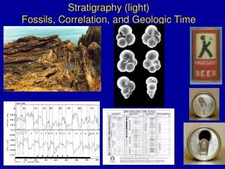
Stratigraphy (light) Fossils, Correlation, and Geologic Time
460 likes | 870 Views
Stratigraphy (light) Fossils, Correlation, and Geologic Time. What kind of ooze is this?. Ooze!!. Planktonic foraminifera Kingdom Protista Subkingdom Protozoa Phylum Sarcomastigophora Subphylum Sarcodina Superclass Rhizopoda Class Granuloreticulosea 28 to 30 extant species.

Stratigraphy (light) Fossils, Correlation, and Geologic Time
E N D
Presentation Transcript
Stratigraphy (light) Fossils, Correlation, and Geologic Time
What kind of ooze is this? Ooze!!
Planktonic foraminifera Kingdom Protista Subkingdom Protozoa Phylum Sarcomastigophora Subphylum Sarcodina Superclass Rhizopoda Class Granuloreticulosea 28 to 30 extant species
Calcareous nannoplankton Includes incerta sedis discoasters Kingdom Chromista Division Heterokonta Class Prymnesiophycae
Radiolaria Diatoms, Kingdom Chromista, Division Haptophyta
Principles of Stratigraphy The holy trinity as blessed by the Heberg bible of stratigraphy is Lithostratigraphy, Chronostratigraphy, and Geochronology. Lithostratigraphy, organization of strata based upon lithologic criteria. Geochronology, abstract time units. Chronostratigraphy, organization of strata based upon age relations – time- rock units Hourglass analogy--duration of sand flow is an hour, but the sand itself is not time
Correlation: establish equivalency Physical correlation establish physical equivalency of unit. Dunbar and Rodgers prefer "physical facies equivalence" "lithocorrelation" Boggs time (temporal) correlation establish equivalence in time of stratigraphic units; often the only meaning implied Physical correlation Principle: Law of Superposition Means of establishing physical correlation
gaps in the record. Derek Ager--more gap than record. Hiatus time gap geochronologic Unconformity: physical break in the record. Chronostratigraphic & lithostratigraphic significance Types: 1) angular unconformity 2) disconformity parallel bedding with erosion 3) paraconformity parallel beds withno evidence of a break 4) Nonconformity strata on non- layered rock
BIOSTRATIGRAPHY: USING FOSSILS TO CORRELATE index fossil, one used in correlation; what are the criteria: zone: fundamental biostratigraphic unit Range zone: based on ranges of one or more taxa narrow stratigraphic range wide environment tolerance unique and identifiable
Interval zones are generally used in construction of biostratigraphic zones that are used for most age correlations Berggren and Miller (1988) planktonic foraminifera
using magnetic field reversals to correlate POWERFUL method of correlation applied to sediments and volcanics why so powerful? Magnetostratigraphy differs from marine magnetic anomalies: Latter fundamental to seafloor spreading, plate tectonics, and construction of geological time scales Magnetostratigraphy
What are the sedimentation rates of the three cores shown? • B/M at <2 m (<3 m/m.y), 4.5 m (~6 m/m.y.), 15.3 m (20 m/m.y.)
Magnetostratigraphy on DSDP/ODP Cores • provided an opportunity for • integration with pelagic • biostratigraphy, isotopic • stratigraphy • this led to the "first testable • time scale" Berggren, • Kent, Flynn, and Van • Couvering (1985) • testable because if we say • the first occurrence of some • foram is in Chron C5n (e.g., Neogloboquadrina acoastensis • can be checked at other • sites versus magstrat.
Correlations Using • Magnetic Susceptibility • J = kH • k = MS = susceptibility • (how "magnetizable" the rocks/ • sediments are) • basalt 10-1 to 10-2 • Sediments 10-3 to 10-5 SI units • (dimensionless) • rapidly measure very closely spaced (cm) • on cores • "pass through" measurement • can be very useful in correlation • proxy of carbonate content • (faster and easier to measure MS) • ODP Leg 138: low carbonate, • more eolian magnetite grains, • therefore higher susceptibilty • proxy of terrigenous versus pelagic
Oxygen Isotopic Stratigraphy Shackleton showed that there is a large component of ice volume in late Pleistocene 18O records. He demonstrated that 18O variations are synchronous and therefore useful for correlation oxygen isotope "stages" (really chrons) 1, 3, 5, 7... are interglacials, 2, 4, 6, 8... are glacials. 4 is a minor glacial. All of other major glaciations 2, 6, 8, back to 20 are spaced roughly 100 k.y. apart
Oxygen isotope/isotopic stratigraphy: Above the SPECMAP time scale 1) is the backbone of the Pleistocene-Recent (Quaternary) time scale and correlations 2) is useful for correlations of older sections 3) provides a "paleo" thermometer 4) provides a proxy for global changes in ice volume
Sr-isotopes Major inputs: 3 primary sources of Sr input into the oceans: oceanic crust, continental crust, and carbonate oceanic crust (basalt) has an average 87Sr/86Sr value of 0.7030 hydrothermal circulation decreases seawater value continental crust (granite composition) 87Sr/86Sr value of 0.720 river input (0.7111) lower due to weathering of limestones (0.707-0.709) carbonate cycle (0.707-0.709) buffers large changes seawater 87Sr/86Sr value is uniform at any given time why? short mixing time of the oceans (1x10³ years) relative to the long residence time of Sr (4x10⁶ years) 87Sr/86Sr values of unaltered marine carbonates reflect seawater 87Sr/86Sr at time of precipitation. why? Strontium substitutes for calcium as a trace element without either strontium isotope being preferentially substituted into the calcium site Burke et al. (1982) used Sr-isotopes as a correlation tool requires a standard seawater curve with which to correlate Sr values and obtain dates
Geochronology “Absolute” ages, “radiometric dates” better said as isotopic age or numerical age Radioactivity: Bequerel (1896) provided Kelvin’s “missing heat” provided a means of numerical estimating ages; chronometer of deep time Isotopic systems generally used to date geological materials K-Ar and Ar-Ar U-Pb Rb-Sr U-Th 14C
Parent Daughter Half life Potassium 40 Argon 40 1.25 billion Rubidium 87 Strontium 87 4.8 x 10¹⁰ years Uranium 235 Lead 207 704 million years Uranium 238 Lead 206 4.47 billion years Thorium 232 Ra 226 1.4 x 10¹⁰ years Thorium 230 Ra 228 75,200 years Carbon 14 Nitrogen 14 5,730 years • Exponential decay (natural log function): • rapid at first, reaches an asymptote; • all follow exponential decay functions: • Radioactive decay, • heat flow (cooling), • subsidence (function of cooling)
Time Scales • Why are time scales important? • provides us with a means of evaluating the relationships of geological data in the time domain • need estimates of rates of processes • in order to establish a precise time scale, all of the requisite temporal correlations must be established • The time scale becomes the ruler against which all geological events & processes are measured.
A "pure" time scale consists of numerous radiometric dates tied to the stratigraphic record • Only good example is the last 4.5 million years: geomagnetic polarity time scale (GPTS) of Cox and Dalrymple • We do not have the luxury of such numerous dates in other parts of the record • Construction of geological time scale requires a ruler to scale time
what is the ruler or vernier for interpolation? biochronology: constant rate of evolution is this assumption ridiculous?? who in their right mind would use this. you do. e.g., 4 ammonite zones in Aptian surprisingly have the same duration. e.g., the Kent and Gradstein (1985) Jurassic time scale that is part of the DNAG first relatively precise Cenozoic time scale (Berggren, 1972) based largely on biochronology magnetochronology assumption of constant sea floor spreading rates between key reversals used for last 160 m.y. Berggren et al., 1985; Cande and Kent, 1992 can do magnetochronology in a sedimentary section, but you assume constant sedimentation rates between magnetochronozonal boundaries plug biostratigraphy, isotopic stratigraphy into magnetostratigraphy "radiochronology" assume constant sedimentation rates between levels with radiometric dates Odin 1982 astrochronology Milankovitch pacemaker provides predicted ages for astronomically forced geological variations
Astrochronology/cyclostratigraphy Sedimentary cycles reflect climatic oscillations that are ultimately controlled by the Earth's orbital cycles. Therefore, sedimentary cycles can be used to construct astronomical time scales. Using this method an astronomical time scale has been established for the late Miocene (6.8-12.0 Ma) to Recent. Such time scales are fundamental to an increasing number of applications in many disciplines. Hilgen, F.J. and Krijgsman, W. (1999). Cyclostratigraphy and astrochronology of the Tripoli diatomite formation (pre-evaporite Messinian, Sicily, Italy), Terra Nova, 11, 16-22. [PDF]
Errors in time correlations • Cenozoic • Biostratigraphy • planktonic foraminifera. widely used. ±0.1 m.y to ±2m.y. typically ±0.5 m.y. • calcareous nannoplankton. widely used. similar resolution as foraminifera • radiolarians. mostly equatorial Pacific. • diatoms. moderately used. not well calibrated to GPTS • Sr-isotopes • late Eocene-Oligocene ±1 to ±0.6 m.y. (at the 95% confidence interval). • Miocene-Recent • 22.8 to 15.6 Ma ±0.6 m.y. (1 analysis @ 95% CI) to ±0.4 m.y. (3 analyses @ 95% CI) 15.2 to ~10 Ma ±1.2 m.y. (1 analysis @ 95% CI) to ±0.8 m.y. (3 analyses @ 95% CI) ca. 10 and 7 Ma, poor resolution. • 7-4.8 Ma ±0.4 m.y. (3 analyses @ 95% CI) • 4.8-2.5 Ma ±1.6 Ma (3 analyses @ 95% CI) • 2.5-0 Ma ±0.3 m.y (3 analyses @ 95% CI) • Magnetostratigraphy • < 10 k.y. when sure of identification of reversal boundary • chrons on the order of 0.2 to 2.6 m.y. (e.g., Chron C24r) duration • hiatuses complicate record • need magnetobiostratigraphy and circular reasoning
Astronomical chronology • 18O has long been primary means of correlation for Bruhnes • resolution as fine as 5-10 k.y. (1/4-1/2 of a precessional cycle) • astronomical time scale complete for the past 10+ m.y. (back through late Miocene) • preliminary astronomical time scale for >10 Ma, 25-33 Ma • pieces being used in older record (e.g., 55-55.5 Ma) • Late Triassic has an astronomical time scale anchored to the basalts (201 Ma) • Mesozoic • Cretaceous • planktonic foraminifera widely used for Late Cretaceous • calcareous nannoplankton. widely used. • ammonites widely used throughout. zones provide better than ±0.5 m.y. relative ages • when present; tied to bentonites in western Interior: “true” (“absolute age”) • chronology can approach << 1m.y. resolution • Jurassic • ammonites widely used throughout. • zones provide better than ±0.5 m.y. relative ages when present • Triassic • ammonites widely used throughout • ________________________________________________ • Paleozoic • bunch of dead brachiopods, conodonts (eel teeth), graptolites (planktonic hemichordates), • trilobites (Cambrian), nautiloids • resolution can be as good as ±0.5 m.y. (relative time); not tied to "real time”