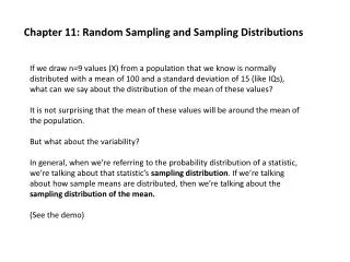
Lecture 10. Random Sampling and Sampling Distributions
Lecture 10. Random Sampling and Sampling Distributions. David R. Merrell 90-786 Intermediate Empirical Methods for Public Policy and Management. Agenda. Normal Approximation to Binomial Poisson Process Random sampling Sampling statistics and sampling distributions

Lecture 10. Random Sampling and Sampling Distributions
E N D
Presentation Transcript
Lecture 10. Random Sampling and Sampling Distributions David R. Merrell 90-786 Intermediate Empirical Methods for Public Policy and Management
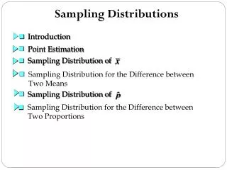
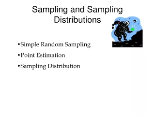
Agenda • Normal Approximation to Binomial • Poisson Process • Random sampling • Sampling statistics and sampling distributions • Expected values and standard errors of sample sums and sample means
Binomial Random Variable Binomial random variable X is the number of “successes” in n trials, where • Probability of success remains the same from trial to trial • Trials are independent
Binomial Probability Distribution Discrete distribution with: • P(X=x) = (n!/(x!(n-x)!))pxqn-x • n is number of trials • x is number of successes in n trials (x = 0, 1, 2, ..., n) • p is the probability of success on a single trial • q is the probability of failure on a single trial
Properties of the Binomial RV • Mean: = np • Variance: = npq • Standard Deviation:
Binomial(n = 10, p = .4) x P(X=x) 0 0.006047 1 0.040311 2 0.120932 3 0.214991 4 0.250823 5 0.200658 6 0.111477 7 0.042467 8 0.010617 9 0.001573 10 0.000105
Approximation to Binomial Distribution • Use normal distribution when: • n is large • np > 10 • n(1 - p) > 10 • Parameters of the approximating normal distribution are the mean and standard deviation from the binomial distribution
Approximation of Binomial Distribution n = 80, p = .4
How Good is the Approximation? Binomial with n = 80 and p = 0.400000 x P( X <= x) 28.00 0.2131 P(X < 29) Normal with mean = 32.0000 and standard deviation = 4.38000 x P( X <= x) 28.0000 0.1806 x P( X <= x) 28.5000 0.2121
Application 1 The Chicago Equal Employment Commission believes that the Chicago Transit Authority (CTA) discriminates against Republicans. The records show that 37.5% of the individuals listed as passing the CTA exam were Republicans; the remainder were Democrats (no one registers as an independent in Illinois). CTA hired 30 people last year, 25 of them were Democrats. What is the probability that this situation could exist if CTA did not discriminate?
Application 1 (cont.) • Success: a Republican is hired • The probability of success, p = 0.375 • The number of trials, n = 30 • The number of successes, x = 5 • P(x 5) = ???
Application 1 (cont.) • Mean: = np = 30*.375 = 11.25 • Variance: = npq = 30*.375*.625 = 7.03 • Standard Deviation: = 2.65 Normal with mean = 11.25 and standard deviation = 2.65 x P( X <= x) 5.5000 0.0150
Poisson Process rate x x x time 0 Assumptions time homogeneity independence no clumping
Poisson Process • Earthquakes strike randomly over time with a rate of = 4 per year. • Model time of earthquake strike as a Poisson process • Count: How many earthquakes will strike in the next six months? • Duration: How long will it take before the next earthquake hits?
Count: Poisson Distribution • What is the probability that 3 earthquakes will strike during the next six months?
Poisson Distribution Count in time period t
Minitab Probability Calculation • Click: Calc > Probability Distributions > Poisson • Enter: For mean 2, input constant 3 • Output: Probability Density Function Poisson with mu = 2.00000 x P( X = x) 3.00 0.1804
Duration: Exponential Distribution • Time between occurrences in a Poisson process • Continuous probability distribution • Mean =1/t
Exponential Probability Problem • What is the probability that 9 months will pass with no earthquake? • t = 1/12, t= 1/3 • 1/ t = 3
Minitab Probability Calculation • Click: Calc > Probability Distributions > Exponential • Enter: For mean 3, input constant 9 • Output: Cumulative Distribution Function Exponential with mean = 3.00000 x P( X <= x) 9.0000 0.9502
Exponential Probability Density Function • MTB > set c1 • DATA > 0:12000 • DATA > end • Let c1 = c1/1000 • Click: Calc > Probability distributions > Exponential > Probability density > Input column • Enter: Input column c1 > Optional storage c2 • Click: OK > Graph > Plot • Enter: Yc2>Xc1 • Click: Display > Connect > OK
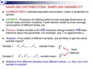
Sampling • Population - entire set of objects that we are interested in studying • Sample - a chosen subset of a population
Some Samples Are ... • random -- each item in the population has an equal chance of being selected to be part of the sample • representative -- has the same characteristics as the population under study, a microcosm of the population
Population Parameters and Sample Statistics • Population Parameter • Numerical descriptor of a population • Values usually uncertain • e.g., population mean (), population standard deviation () • Sample Statistics • Numerical descriptor of a sample • Calculated from observations in the sample • e.g., sample mean , sample standard deviation S
What is a sampling distribution? • Sample statistics are random variables • Sample statistics have probability distributions • “Sampling distribution” is the probability distribution of a sample statistic
MTB > Retrieve 'C:\MTBWIN\DATA\RESTRNT.MTW'. Retrieving worksheet from file: C:\MTBWIN\DATA\RESTRNT.MTW Worksheet was saved on 5/31/1994 MTB > info Information on the Worksheet Column Name Count Missing C1 ID 279 0 C2 OUTLOOK 279 1 C3 SALES 279 25 C4 NEWCAP 279 55 C5 VALUE 279 39 C6 COSTGOOD 279 42 C7 WAGES 279 44 C8 ADS 279 44 C9 TYPEFOOD 279 12 C10 SEATS 279 11 C11 OWNER 279 10 C12 FT.EMPL 279 14 C13 PT.EMPL 279 13 C14 SIZE 279 16
MTB > desc 'sales' Descriptive Statistics Variable N N* Mean Median TrMean StDev SEMean SALES 254 25 332.6 200.0 248.9 650.5 40.8 Variable Min Max Q1 Q3 SALES 0.0 8064.0 83.7 382.7 MTB > boxp 'sales' * NOTE * N missing = 25
MTB > hist 'sales' * NOTE * N missing = 25
MTB > let c15 = loge('sales') MTB > let c15 = loge('sales') J *** Values out of bounds during operation at J Missing returned 1 times MTB > let c15 = loge('sales' + 1) MTB > name c15 'logsales' MTB > desc 'logsales' Descriptive Statistics Variable N N* Mean Median TrMean StDev SEMean logsales 254 25 5.1830 5.3033 5.2134 1.1387 0.0715 Variable Min Max Q1 Q3 logsales 0.0000 8.9953 4.4394 5.9500 MTB > boxp 'logsales' * NOTE * N missing = 25
Four Samples of Size 50 From Restaurant “Logsales” Data--Histograms
Random Samples from Restaurant “Logsales” Data--Summary MTB > Desc c16-c19 Descriptive Statistics Variable N N* Mean Median TrMean StDev SEMean C16 43 7 5.246 5.375 5.280 0.867 0.132 C17 43 7 5.351 5.352 5.383 1.223 0.186 C18 48 2 5.366 5.461 5.388 0.888 0.128 C19 43 7 5.244 5.198 5.253 0.937 0.143 Variable Min Max Q1 Q3 C16 2.773 6.621 4.625 5.787 C17 1.099 8.456 4.710 6.176 C18 2.485 7.091 4.961 5.994 C19 3.434 6.868 4.595 6.089
Next Time ... • Central Limit Theorem--”Sample averages are approximately normally distributed”