Sampling distributions:

1. Sampling distributions:

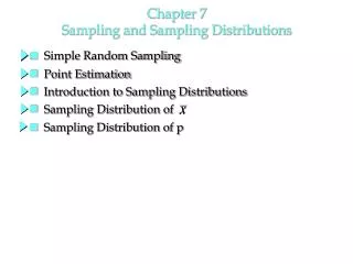
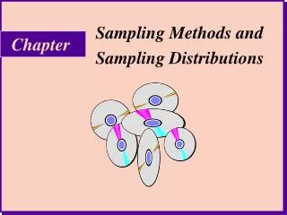
2. In Psychology we generally make inferences about populations on the basis of samples. We therefore need to know what relationship exists between samples and populations. A population of scores has: mean (μ), standard deviation (σ) and shape (e.g., normal distribution).

3. CONCRETE BUT MUNDANE EXAMPLE: HEIGHT OF ALL ADULT WOMEN IN ENGLAND high µ = 63 in. σ = 2 in. frequency of raw scores σ low 63 67 59 61 65 Height (inches)

4. Sample of 100 adult women from England high s = 2.5 in N = 100 frequency of raw scores s low 64.2 in

5. If we take repeated samples, each sample has a mean height ( ), a standard deviation (s), and a shape. Due to random fluctuations, each sample is different - from other samples and from the parent population. Fortunately, these differences are predictable - and hence we can still use samples in order to make inferences about their parent populations.

6. Taking multiple samples (of a given size) gives rise to: Sampling Distribution Frequency (how many means of a given value) 63.0 Mean sample heights (inches)

7. What are the properties of the distribution of Sample Means (Sampling Distribution)? (a) The mean of the sample means is the same as the mean of the population of raw scores: (b) The sampling distribution of the mean also has a standard deviation. The standard deviation of the sample means is called the "standard error". It is NOT the same as the standard deviation of the population (of raw scores).

8. The standard error is smaller than the population SD: The bigger the sample size, the smaller the standard error. i.e., variation between samples decreases as sample size increases. (This is because sample mean based on a large sample reduces the influence of any extreme raw scores in a sample.)

9. Suppose we take samples of N = 100 Sampling distribution for N = 100 µ = 63 in. N = 100 frequency 63 Mean sample heights (inches)

10. How do we calculate the standard deviation of a sampling distribution of the mean (known as the standard error)? For N =100 Suppose the N = 16 instead of 100

11. (c) -The distribution of sample means is normally distributed if the population of scores is normally distributed. - The distribution of sample means (for N ≥ 30) is normally distributed no matter what the shape of the original distribution of raw scores is!

12. Example: Annual income of Americans. Many people in the lower and medium income bracket; very few are ultra rich. (So distribution is NOT normal.) Suppose we take many samples of size N = 50. The sampling distribution of the mean will be normal. This is due to the Central Limit Theorem.

13. Given the distribution is normal, we use properties of normal distribution to do interesting things. Various proportions of scores fall within certain limits of the mean (i.e. 68% fall within the range of the mean +/- 1 standard deviation; 95% within +/- 2 standard deviation, etc.).

14. Quick reminder about z-scores With a z-score, we can represent a given score in terms of how different it is from the mean of a distribution of scores. μ = 63 Xi = 64 Calculating z-score

15. Relationship of a sample mean to the population mean: μ = 63 64 We can do the same with sample means: (a) we obtain a particular sample mean; (b) we can represent this in terms of how different it is from the mean of its parent population.

16. If we obtain a sample mean that is much higher or lower than the population mean, there are two possible reasons: (a) our sample mean is a rare "fluke" (a quirk of sampling variation); (b) our sample has not come from the population we thought it did, but from some other, different, population. The greater the difference between the sample and population means, the more plausible (b) becomes.

17. Take another example: The human population IQ mean is 100. A random sample of people has a mean IQ of 170. There are two explanations: (a) the sample is a fluke: by chance our random sample contained a large number of highly intelligent people. (b) the sample does not come from the population we thought it did: our sample was actually from a different population - e.g., aliens masquerading as humans. Or, more likely, it was taken from the Mensa society members.

18. Relationship between population mean and sample mean: high frequency of sample means low population mean IQ = 100 sample mean IQ = 170

19. This logic can be extended to the difference between two samples from the same population: A common experimental design We compare two groups of people: - One group get the "wolfman" drug (Experimental group). - The second group get a placebo (Control group). At the start of the experiment, they are two samples from the same population ("humans").

20. At the end of the experiment, are they: (a) still two samples from the same population (i.e., still two samples of "humans" – i.e. our experimental treatment has left them unchanged). OR (b) now samples from two different populations - one from the "population of humans" and one from the "population of wolfmen"?

21. We can decide between these alternatives as follows: The differences between any two sample means from the same population are normally distributed, around a mean difference of zero. Most differences will be relatively small, since the Central Limit Theorem tells us that most samples will have similar means to the population mean (and hence similar means to each other). If we obtain a very large difference between our sample means, it could have occurred by chance, but this is very unlikely - it is more likely that the two samples come from different populations.

22. Possible differences between two sample means: a big difference between mean of sample A and mean of sample B: high frequency of raw scores low mean of sample A mean of sample B low high sample means

23. Possible differences between two sample means (cont.): a small difference between mean of sample A and mean of sample B: high frequency of raw scores low mean of sample A mean of sample B high low sample means

24. Frequency distribution of differences between sample means: high frequency of differences between sample means low mean A smaller than mean B mean A bigger than mean B no difference size of difference between sample means ( "sample mean A" minus "sample mean B")

25. Frequency distribution of differences between sample means: A small difference between sample means (quite likely to occur by chance) high frequency of differences between sample means low mean A bigger than mean B mean A smaller than mean B no difference size of difference between sample means

26. Frequency distribution of differences between sample means: high A large difference between sample means (unlikely to occur by chance) frequency of differences between sample means low mean A bigger than mean B mean A smaller than mean B no difference size of difference between sample means