 Physics opportunities at the beginning  Machine start-up scenario

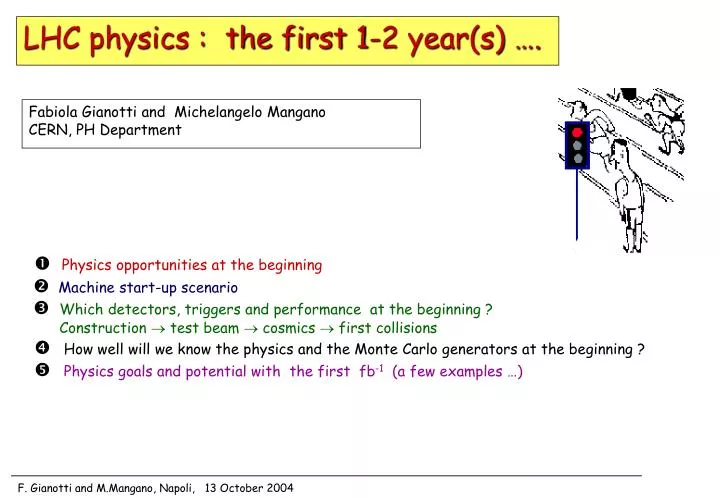
1. LHC physics : the first 1-2 year(s) …. Fabiola Gianotti and Michelangelo Mangano CERN, PH Department  Physics opportunities at the beginning  Machine start-up scenario  Which detectors, triggers and performance at the beginning ? Construction  test beam  cosmics  first collisions  How well will we know the physics and the Monte Carlo generators at the beginning ? Physics goals and potential with the first fb-1 (a few examples …)

2. What can we reasonably expect from the first year(s)?Some history: -- Fall 1982: first physics run for UA1 and UA2 at the SppbarS Lmax=5x1028cm-2s-1 ≈ 1% asymptotic L Lint = 20nb-1 in 30 days outcome: W/Z discovery, as expected ingredients: plenty of kinematical phase-space (ISR was sub-threhsold!), clear signature, and good hands-on control of backgrounds-- Summer 1987: first physics run for CDF at the Tevatron Lmax=5x1028cm-2s-1 ≈ 1% nominal L Lint = 20nb-1 in 30 days outcome: nothing exciting,as expected why: not enough phase-space, given the strong constraints on new physics already set by UA1/UA2!

3. In the region of the UA1 limit the production cross-section at the Tevatron was only a factor of 10-20 larger By the time of CDF startup, the SppS had already logged enough luminosity to rule out a possible observation at the Tevatron within the first 100nb-1 It took 2 more years (and 4pb-1) for CDF to improve (mtop>77 GeV) the UA1 limits (in spite of the fact that by ‘89, and with 5pb-1, had only improved to 60 GeV - UA2 eventually went up to 69 GeV). This is the consequence of much higher bg’s at the Tevatron, and of the steep learning curve for such a complex analysis

4. At the start of LHC, the situation will resemble much more that at the beginning of UA1/UA2: The phase-space for the Tevatron will have totally saturated the search boundary for most phenomena, at a level well below the LHC initial reach: seen from the LHC, the Tevatron will look like the ISR as seen from the SppS! Rates 103 times larger in the region of asymptotic Tevatron reach 1% of Lmax for the LHC, (as in SppS and Tevatron early runs), close to Lmax for Tevatron (assume a 1% signal efficiency) N.B.: rates for gluino production are roughly a factor of 10 larger than for HQs

5. Similar considerations hold for jets, where few days of data will probe quarks at scales beyond the overall Tevatron CM energy!

6. Fine, we have phase-space, we have rates. But should we truly expect something to show up at scales reachable early on? LEP’s heritage is a strong confirmation of the SM, and at the same time an apparent paradox: on one side m(H)=117+45-68; on the other, SM radiative corrections give How can counterterms artificially conspire to ensure a cancellation of their contribution to the Higgs mass? The existence of new phenomena at a scale not much larger than 400 GeV appears necessary to enforce such a cancellation in a natural way! The accuracy of the EW precision tests at LEP, on the other hand, sets the scale for “generic new physics” (parameterized in terms of dim-5 and dim-6 effective operators) at the level of few-to-several TeV. This sets very strong constraints on the nature of this possible new physics: to leave unaffected the SM EW predictions, and at the same time to play a major role in the Higgs sector. Supersymmetry offers one such possible solution

7. Heinemeyer In Supersymmetry the radiative corrections to the Higgs mass are not quadratic in the cutoff, but logarithmic in the size of SUSY breaking (in this case Mstop/Mtop): with For Msusy< 2TeV The current limits on mH point to M(lightest stop) > 600 GeV. Pushing the SUSY scale towards the TeV, however, forces fine tuning in the EW sector, reducing the appeal of SUSY as a solution to the Higgs mass naturalness:

8. In other words, the large value of mH shows that room is getting very tight now for SUSY, at least in its “minimal” manifestations. This makes the case for an early observation of SUSY at the LHC quite compelling, and worth investing into! For some people the room left is too tight. Some skepticism on SUSY has emerged, and a huge effort of looking for alternatives has began few years back, leading to a plethora of new ideas (Higgless-models, Little Higgs, extra-dimensions, etc) Some of these ideas lead to rather artificial structures, where the problem of the Higgs naturalness is shifted to slightly higher scales, via the introduction of a new sector of particles around the TeV. The observation of new phenomena within the first few yrs of run, in these cases, is not guaranteed (nor is it asymptotically) Few of these scenarios offer the appeal of Supersymmetry, with its clear predictions (calculability), and connections with the other outstanding problems of the Standard Model (Dark Matter, Flavour, CP violation)

11. photons+MET (gauge mediated SUSY) The search for Supersymmetry is in my view the single most important task facing the LHC experiments in the early days. In several of its manifestations, SUSY provides very clean final states, with large rates and potentially small bg’s. Jets + miss ET (squarks/gluinos) Same-sign dileptons + MET (gluinos) Bs->mu+mu- t tbar+ MET (stop production) Given the big difficulty and the low rates characteristic of Higgs searches in the critical domain mH<135 GeV, I feel that the detector and physics commissioning should be optimized towards the needs of SUSY searches rather than light-Higgs (I implicitly assume that for mH>140 Higgs searches will be almost staightforward and will require proper understanding of only a limited fraction of the detector components -- e.g. muons)

12. The early determination of the scale at which new physics manifests itself will have important consequences for the planning of facilities beyond the LHC (LC? CLIC? nufact? Flavour factories? Underground Dark Matter searches?). The LHC will have no competition in the search for new physics, so in principle there is no rush. But the future of the field will greatly benefit from a quick feedback on SUSY and the rest!

13. ~ 400 dipoles delivered ~ 300 cold-tested  see L.Rossi Machine start-up scenario (from Chamonix XII Workshop, January 2003) ~ April 2007 : start machine cool-downfollowed by machine commissioning (mainly with single beam) ~ Summer 2007 : two beams in the machine  first collisions -- 43 + 43 bunches, L=6 x 1031 cm-2 s-1(possible scenario; tuning machine parameters) -- pilot run: 936+936 bunches (75 ns  no electron cloud), L>5x 1032 -- 2-3 month shut-down ? -- 2808 + 2808 bunches (bunch spacing 25 ns), L up to ~2x1033 (goal of first year)  ~ 7 months of physics run A lot of uncertainties in this plan (QRL !)  here show potential vs integrated luminosity from ~ 100 pb-1 /expt to ~ 10 fb-1 /expt

14. RPC over ||<1.6 (instead of ||< 2.1) 4th layer of end-cap chambers missing 2 pixel layers/disks instead of 3 TRT acceptance over ||< 2 (instead of ||< 2.4)  Which detectors the first year(s)? Pixels and end-cap ECAL installed during first shut-down Both experiments: deferrals of high-level Trigger/DAQ processors  LVL1 output rate limited to ~ 50 kHz CMS (instead of 100 kHz) ~ 35 kHz ATLAS (instead of 75 kHz) Impact on physics visible but acceptable Main loss : B-physics programme strongly reduced (single  threshold pT> 14-20 GeV)

15. blue : few hours of minimum bias CMS ECAL Expected performance day 1 Physics samples to improve (examples) ECAL uniformity ~ 1% (ATLAS), 4% (CMS) Minimum-bias, Z ee e/ scale 1-2 % ? Z  ee HCAL uniformity 2-3 % Single pions, QCD jets Jet scale < 10% Z ( ll) +1j, W  jj in tt events Tracking alignment 20-500 m in R ? Generic tracks, isolated m , Z  mm Which detector performance at day one ? A few examples and educated guesses based on test-beam results and simulation studies Ultimate statistical precision achievable after few days of operation. Then face systematics …. E.g. : tracker alignment : 100 mm (1 month)  20mm (4 months)  5 mm (1 year) ?

16. Test-beam  E- resolution ATLAS HAD end-cap calo Geant4 G4 G3 data Longitudinal profile of 100 GeV test-beam pions in CMS HCAL ~ 70% /E Steps to achieve the detector goal performance • Stringent construction requirements and quality controls (piece by piece …) • Equipped with redundant calibration/alignment hardware systems • Prototypes and part of final modules extensively tested with test beams • (allows also validation of Geant4 simulation) • In situ calibration at the collider (accounts for material, global detector, B-field, long-range mis-calibrations and mis-alignments) includes : -- cosmic runs : end 2006-beg 2007 during machine cool-down • -- beam-gas events, beam-halo muons during single-beam period • -- calibration with physics samples (e.g. Z ll, tt, etc.)

17. 100 fb-1 Example of this procedure : ATLAS electromagnetic calorimeter Pb-liquid argon sampling calorimeter with Accordion shape, covering || < 2.5 H   : to observe signal peak on top of huge  background need mass resolution of ~ 1%response uniformity (i.e. total constant term of energy resolution)  0.7% over || < 2.5

18. Construction phase (e.g. mechanical tolerances):  287 GeV electron response variation with Pb thickness from ‘93 test-beam data < > = 2.2 mm   9 m 1% more lead in a cell  0.7% response drop  to keep response uniform to 0.2-0.3%, thickness of Pb plates must be uniform to 0.5% (~ 10 mm) Thickness of all 1536 absorber plates (1.5m long, 0.5m wide) for end-cap calorimeter measured with ultrasounds during construction

19. Beam tests of 4 (out of 32) barrel modules and 3 (out of 16) end-cap modules:  • 1 barrel module: •  x  = 1.4 x 0.4 • ~ 3000 channels Scan of a barrel module with 245 GeV e-   r.m.s.  0.57% over ~ 500 spots Uniformityover “units” of size  x  = 0.2 x 0.4 :~ 0.5% 400 such units over the full ECAL

20. Check calibration with cosmic muons:  Through-going muons ~ 25 Hz (hits in ID + top and bottom muon chambers) Pass by origin ~ 0.5 Hz (|z| < 60 cm, R < 20 cm, hits in ID) Useful for ECAL calibration ~ 0.5 Hz (|z| < 30 cm, E cell > 100 MeV, ~ 900 ) From full simulation of ATLAS (including cavern, overburden, surface buildings) + measurements with scintillators in the cavern: Cosmic muons in ATLAS pit in 0.01 s …. • ~ 106 events in ~ 3 months of data taking • enough for initial detector shake-down (catalog problems, gain operation experience, some alignment/calibration, detector synchronization, …)

21. Muon signal in barrel ECAL Test-beam data S() / (noise) 7 0.15 % / nH Test-beam data  Precision of ECAL readout calibration system : 0.25%. But : -dependent differences between calibration and physics signals • can be checked with cosmic muons From studies with test-beam muons: can check (and correct) calorimeter response variation vs  to 0.5% in < 3 months of cosmics runs Note : not at level of ultimate calibration uniformity (~ 0.25%) but already a good starting point

22.  First collisions : calibration with Z  ee events rate ~ 1 Hz at 1033, ~ no background, allows ECAL standalone calibration Use Z  ee events and Z-mass constraint to correct long-range non-uniformities. From full simulation : ~ 250 e /unit needed to achieve cLR  0.4%  ctot = 0.5%  0.4%  0.7% ~ 105 Z  ee events (few days of data taking at 1033) ctot = cL cLR cL 0.5% demonstrated at the test-beam over units  x  = 0.2 x 0.4 cLR long-range response non-uniformities from unit to unit (400 total) (module-to-module variations, different upstream material, etc.) • Nevertheless, let’s consider the worst (unrealistic ?) scenario : no corrections applied • cL = 1.3 % measured “on-line” non-uniformity of individual modules • cLR = 1.5 % no calibration with Z  ee ctot 2% conservative : implies very poor knowledge of upstream material (to factor ~2) H   significance mH~ 115 GeV degraded by ~ 25%  need 50% more L for discovery

23. How well will we know LHC physics on day one (before data taking starts ) ? * DY processes * top X-sections * bottom X-sections * jet X-sections * Higgs X-sections

24. MLM, Frixione W/Z cross-sections Theory OK to 2% + 2%(PDF) Similar accuracy for high-mass DY (bg, as well as signal, for massive Z’/W’)

25. tt cross-section tt FNAL= 6.5pb (1 ± 5%scale ± 7%PDF ) Scale unc: ± 12%NLO => ± 5%NLO+NLL ) Ds = ± 6% => Dm= ± 2 GeV tt LHC= 840pb (1 ± 5%scale ± 3%PDF )

26. ✫ ✫ ✫ ✫ 150 ✫ ✫ ✫ ✫ ✫ 140 ✫ 130 ✫no UE subtraction 120 ▲ UE subtraction 1.4 0.8 1.2 ΔRclus Recent overview of ATLAS strategy and results for mtop: hep-ph/0403021 Channels considered: + (W-> lnu)+4 jets, 2 b tags + high-pT top, t->3 jets + (W->lnu) (W->lnu) + bb + m(l-psi) in events with B->psiX Need a strategy for validation of the MC input models: + UE modeling and subtraction + validation of FSR effects: * jet fragmentation properties, jet energy profiles * how do we validate emission off the top quark in the high-pt top sample? * b fragmentation function

27. bb cross-sections OK, but theoretical systematics still large: +-35% at low pt +-20% for pt>>mb In view of the recent run II results from CDF, more validation required. To verify the better predictivity at large pt, need to perform measurements in the region 30-80 geV, and above (also useful to study properties of high-Et b jets, useful for other physics studies)

28. Higgs cross-sections NNLO available for dominant gg->H process => almost as accurate as DY PDF uncert sufficient for day-1 business, but improvements necessaryfor high-lum x-sec studies (=>to measure couplings)

29. Jet cross-sections Theoretical syst uncertainty at NLO ~ +-20% PDF uncert (mostly g(x)) growing at large x

30. DO, run I data Puzzling discrepancy at low ET, in view of the fact that at NLO rates for cone-jets with R=0.7 and kT jets with D=1 are equal to within 1% OK at high-ET

31. Main sources of syst uncertainties (CDF, run I) At high ET the syst is dominated by the response to high pT hadrons (beyond the test beam pT range) and fragmentation uncertanties Out to which ET will the systematics allow precise cross-section measurements at the LHC? Out to which ET can we probe the jet structure (multiplicity, fragm function)? NB: stat for Z+jet or gamma+jet runs out before ET~500 GeV

32. Z+jet gamma+jet

34. Extrapolation from Tevatron to LHC is hard, as it relies on the understanding of the unitarization of the minijet cross-section • The mini-jet nature of the UE implies that the particle and energy flows are not uniformly distributed within a given event:can one do better than the standard uniform, constant, UE energy subtraction? • Studies of MB and UE should be done early on, at very low luminosity, to remove the effect of overlapping pp events: • MB triggers • low-ET jet triggers

35.  Physics goals and potential in the first year (a few examples ….) ~ few PB of data per year per experiment  challenging for software and computing (esp. at the beginning …) assuming 1% of trigger bandwidth Already in first year, large statistics expected from: -- known SM processes understand detector and physics at s = 14 TeV -- several New Physics scenarios Note: overall event statistics limited by ~ 100 Hz rate-to-storage ~ 107 events to tape every 3 days assuming 30% data taking efficiency

36. Goal # 1 t Goal # 2 t Goal # 3 Understand and calibrate detector and trigger in situ using well-known physics samples e.g. - Z  ee,  tracker, ECAL, Muon chambers calibration and alignment, etc. - tt  bl bjj 103 evts/day after cuts jet scale from Wjj, b-tag perf., etc. Understand basic SM physics at s = 14 TeV first checks of Monte Carlos (hopefully well understood at Tevatron and HERA) e.g. - measure cross-sections for e.g. minimum bias, W, Z, tt, QCD jets (to ~ 10-20 %), look at basic event features, first constraints of PDFs, etc. - measure top mass (to 5-7 GeV) give feedback on detector performance Note : statistical error negligible after few weeks run Prepare the road to discovery: -- measure backgrounds to New Physics : e.g. tt and W/Z+ jets (omnipresent …) -- look at specific “control samples” for the individual channels: e.g. ttjj with j  b “calibrates” ttbb irreducible background to ttH  ttbb Look for New Physics potentially accessible in first year (e.g. Z’, SUSY, some Higgs ? …)

37. Use gold-plated tt  bW bW  bl bjj channel • Very simple selection: • -- isolated lepton (e, ) pT > 20 GeV • -- exactly 4 jets pT > 40 GeV • -- no kinematic fit • -- no b-tagging required (pessimistic, • assumes trackers not yet understood) • Plot invariant mass of 3 jets with highest pT ATLAS 150 pb-1 ( < 1 week at 1033) B=W+4 jets (ALPGEN MC) M (jjj) GeV Example of initial measurement : top signal and top mass Events at 1033 • top signal visible in few days also with • simple selections and no b-tagging • cross-section to ~ 20% (10% from luminosity) • top mass to ~7 GeV (assuming b-jet scale to 10%) • get feedback on detector performance : -- mtop wrong  jet scale ? -- gold-plated sample to commission b-tagging

38. Already with 30 pb-1 ATLAS 150 pb-1 ATLAS 150 pb-1 Fit signal and background (top width fixed to 12 GeV)  extract cross-section and mass Can we see a W  jj peak ? Select the 2 jets with highest pT (better ideas well possible …) W peak visible in signal, no peak in background

39. no b-tag Introduce b-tagging …. ATLAS 150 pb-1 Bkgd composition changes: combinatorial from top itself becomes more and more important 1 b-tag + cut on W-mass window 2 b-tags + cut on W-mass window

40. What about early discoveries ? • An easy case : a new resonance decaying into e+e-, e.g. a Z ’  ee of mass 1-2 TeV • An intermediate case : SUSY • A difficult case : a light Higgs (m ~ 115 GeV)

41. Z ’  ee, SSM Mass Expected events for 10 fb-1L dt needed for discovery (after all cuts) (corresponds to 10 observed evts) 1 TeV ~ 1600 ~ 70 pb-1 1.5 TeV ~ 300 ~ 300 pb-1 2 TeV ~ 70 ~ 1.5 fb-1 ATLAS, 10 fb-1, barrel region An “easy case” : Z’ of mass 1-2 TeVwith SM-like couplings • signal rate with L dt ~ 0.1-1 fb-1large enough • up to m  2 TeV if “reasonable” Z’ee couplings • dominant Drell-Yan background small • (< 15 events in the region 1400-1600 GeV, 10 fb-1) • signal as mass peak on top of background • Z  ll +jet samples and DY needed for E-calibration • and determination of lepton efficiency

42. Large cross-section   100 events/dayat 1033 for Spectacular signatures  SUSY could be found quickly 5 discovery curves q ~ one year at 1034: up to ~2.5 TeV q 02 ~ one year at 1033 : up to ~2 TeV Z 01 ~ one month at 1033 : up to ~1.5 TeV cosmologically favoured region Tevatron reach : < 500 GeV An intermediate case : SUPERSYMMETRY Using multijet + ETmiss (most powerful and model-independent signature if R-parity conserved) Measurement of sparticle masses likely requires > 1 year. However …

43. Peak position correlated to MSUSY Events for 10 fb-1 background signal Events for 10 fb-1  Tevatron reach ATLAS ET(j1) > 80 GeV ETmiss > 80 GeV signal background From Meff peak first/fast measurement of SUSY mass scale to  20%(10 fb-1, mSUGRA) Detector/performance requirements: -- quality of ETmiss measurement (calorimeter inter-calibration/linearity, cracks)  apply hard cuts against fake MET and use control samples (e.g. Z  ll +jets) -- “low” Jet / ETmiss trigger thresholds for low masses at overlap with Tevatron region (~400 GeV)

44. Background processControl samples (examples ….) (examples ….) Z ( ) + jetsZ ( ee, ) + jets W ( ) + jets W ( e, ) + jets tt blbjjtt bl bl QCD multijetslower ET sample normalization point D0 DATA MC (QCD, W/Z+jets) 2 “e” +  1jet sample Backgrounds will be estimated using data (control samples) and Monte Carlo: Can estimate background levels also varying selection cuts (e.g. ask 0,1,2,3 leptons …) A lot of data will most likely be needed ! normalise MC to data at low ET miss and use it to predict background at high ET miss in “signal” region • Hard cuts against fake ET miss : • reject beam-gas, beam-halo, • cosmics • - primary vertex in central region • - reject event with ETmiss vector • along a jet or opposite to a jet • reject events with jets in cracks • etc. etc.

45. Can we trust the current estimates of bg rates?

46. Njet≥4 ET(1,2)>100 GeV ET(3,4)>50 GeV MET>max(100,Meff/4) Meff=MET+∑ETj “Correct” bg shape indistinguishable from signal shape!

47. fb-1 Meff Use Z->ee + multijets, apply same cuts as MET analysis but replace MET with ET(e+e-) Extract Z->nunu bg using, bin-by-bin: (Z->nunu) = (Z->ee) B(Z->nunu)/B(Z->ee) Assume that the SUSY signal is of the same size as the bg, and evaluate the luminosity required to determine the Z->nunu bg with an accuracy such that: Nsusy > 3 sigma where sigma=sqrt[ N(Z->ee) ] * B(Z->nunu)/B(Z->ee) => several hundred pb-1 are required. They are sufficient if we believe in the MC shape (and only need to fix the overall normalization). Much ore is needed if we want to keep the search completely MC independent How to validate the estimate of the MET from resolution tails in multijet events??

48. here discovery easier with H  4l mH > 114.4 GeV H  ttH  ttbbqqH  qq (ll + l-had) S 13015~ 10 B 4300 45~ 10 S/ B2.02.2~ 2.7 ATLAS total S/ B K-factors  (NLO)/(LO)  2 not included A difficult case: a light Higgs mH ~ 115 GeV mH ~ 115 GeV 10 fb-1 Full GEANT simulation, simple cut-based analyses

49. H   ttH  tt bb  bl bjj bb qqH  qq b b  H  Remarks: Each channel contributes ~ 2 to total significance  observation of all channels important to extract convincing signal in first year(s) The 3 channels are complementary robustness: • different production and decay modes • different backgrounds • different detector/performance requirements: • -- ECAL crucial for H   (in particular response uniformity) : /m ~ 1% needed • -- b-tagging crucial for ttH : 4 b-tagged jets needed to reduce combinatorics • -- efficient jet reconstruction over || < 5 crucial for qqH  qq : • forward jet tag and central jet veto needed against background Note : -- all require “low” trigger thresholds E.g. ttH analysis cuts : pT (l) > 20 GeV, pT (jets) > 15-30 GeV -- all require very good understanding (1-10%) of backgrounds

50. Luminosity needed for 5s discovery (ATLAS+CMS) CMS , 10 fb-1 Signal Backgr. Events / 0.5 GeV H  4l (l=e,) m (4l) If mH > 180 GeV : early discovery may be easier with H  4l channel • H  WW  l l : high rate (~ 100 evts/expt) but no mass peak not ideal for early discovery … • H  4l : low-rate but very clean : narrow mass peak, small background • Requires: -- ~ 90% e,  efficiency at low pT (analysis cuts : pT 1,2,3,4 > 20, 20, 7, 7, GeV) • --  /m ~ 1%, tails < 10% good quality of E, p measurements in ECAL and tracker