Download
1 / 66
660 likes | 793 Views
Explore the uncertainty in moment tensor calculations, from linear problems to non-gaussian errors, using SVD for a transparent expression of uncertainty. Learn about ISOLA for probabilistic location and linear problem solutions, with practical examples. Improve your understanding of error volumes in a non-linear problem setting.

E N D
Estimating uncertainty of moment tensor using singular vectors. J. Zahradník Charles University in Prague Czech Republic
Motivation The cases exist that MT was successfully derived from a few stations. When and why? The volume component is highly unstable. How does it trade-off with the other MT components? How to solve these questions without seismograms?
Part 1 Theory (Numerical Recipes, chap. 2.6, 15.4, 15.6)
Linear problem, least squares, solution by means of normal equations. Cautionr: data variance needed!
Linear problem, least squares, solution by means of SVD. Advantage: SVD expresses the uncertainty by singular vectors in a transparent way. Cautionr: data variance needed!
Gaussian and non-gaussian errors Non-linear problems and non-gaussian errors: ! Ellipsoid substituted by an irregular (perhaps non-compact) error volume. The probability density function (pdf) has to be found experimentally.
Example what cannot be used if errors are non-gaussian. In gaussian case the absolute size of the confidence interval can be found (related to a given probability level) if we know the covariance matrix. In practice, however, we often do not know data errors, so the covariance still cannot be used (even for gaussian errors) in absolute sense….
Example of error volumes of a non-linear problem. Probabilistic location (NonLinLoc, A. Lomax) Highly important even in a relative sense (without exact knowledge of the data errors)! Epicenter (2 parameters) Depth (1 single parameter may have a specific physical meaning) V. Plicka
Part 2 Linear problem for MT (position and source time fixed) Motivation: Greece -Dana Křížová Portugal - Susana Custódio
Uncertainty in practice: 10/5/2008 4 agencies may represent 4 solutions (for some events) Instituto Andaluz de Geofísica (IAG) Instituto Geográfico Nacional (IGN) OBS stations (NEAREST) Ana Lúcia das Neves Araújo da Silva Domingues (red beachballs)
Example to study the MT uncertainty ISOLA ISOLA old: a) min/max eigenvalue ratio of the matrix of normal equations b) Variances of the parameters a1,…a6 ISOLA new: ??????????????
ISOLA new: • Perturbing the MT solution • within the error ellipsoid • We need: crustal model, station positions, • source position, and also the assumed MT. • We do not need neither the true MT, nor seismograms. • ISOLA produces the matrix, the singular vectors and values, and an auxiliary code generates the ellipsoid.
6 stations, source depth 10 km Ellipsoid for delta chi^2=1: for 1D pdf and gaussian errors it is equivalent to +/- 1 sigma. The star delta ai= 0 is the given MT. Presented is a 2D section, but we calculate a 6D elipsoid, a1…a6.
Perturbing mechanism: Strike = 106°, Dip = 11° , Rake = 153° Strike = 222°, Dip = 85° , Rake = 80° VOL 9% f < 0.2 Hz 6 stations, source depth 10 km Each point = a point inside the ellipsoid of chi^2=1. (colors unimportant)
6 stations, source depth 10 km vectors are in coloumns, each row is one component Singular vector almost parallel to a6. + + + + + • s(a6) and how it is made up s(a6) … the largest parameter uncertainty
an extreme case of 1 station, source depth 60 km
Perturbing mechanism: Strike = 106°, Dip = 11° , Rake = 153° Strike = 222°, Dip = 85° , Rake = 80° VOL 9% f < 0.2 Hz 1 station, source depth 60 km
1 station, source depth 60 km At least 2 vectors are ‘in the play’, with dominant components along a1, a4, a6
1 station, source depth 10 km Perturbing mechanism: Strike = 106° Dip = 11° Rake = 153° 1 station, source depth 60 km
6 stations, source depth 10 km Perturbing mechanism: Strike = 106° Dip = 11° Rake = 153° 6 stations, source depth 60 km
Attention ! Even the MT itself is important… We can apply the same ellipsoid to perturb a different MT [i.e. to study uncertainty of an earthquake of a different mechanism] if the source position and stations remain the same. (Reason: The problems is linear in a1, … a6.)
1 station, source depth 10 km • Perturbing the former mechanism: • Strike dip rake • 11 153 • 222 85 80 153 80 marks a problem • 1 station, source depth 10 km • Perturbinganother • mechanism • 74 -15 • 75 -163 • Note a different • uncertainty, • e.g. better rake … • no problem like above)
Possible outlook The cases may exist when MT can be determined from a very few stations (Mars ??, forensic seismology??). Possibility to design network extension, e.g. where to put efficient OBS.
Many factors are not included in this analysis, mainly the uncertainty of the crustal model. And the noise! For example, when combining the land and ocean bottom stations, one should count with higher noise of the latter. Etc. ….
Part 3 Volume component Great advantage of the MT inversion formulated by means of the basis mechanisms like in ISOLA: Note that VOL is given by a single parameter, just a6. Mkk = a6. 6 basis mechanisms
Multiple DC a single full MT (apparent VOL 16% due to neglecting finite extent) color green circles Gallovič & Zahradník (submitted)
We use synthetics of the single-source Myiagi as a model of the seismogram with a known VOL component(although it is only apparent VOL).
= SIGMA from isola (incl. vardat) .257820E-01 .954336E-01 .415202E-01 .381398E-01 .438742E-01 .495832E-01 s(a6) was already in ISOLA old, but here we learn about trade off between different parameters within the 6D ellipsoid.
VOL % : 16.4, DC % : 57.4, CLVD % : 26.2 strike,dip,rake: 206 32 101 strike,dip,rake: 12 58 82 source depth 3.9 km 12 stations, f< 0.2 Hz data variance=0.01 m2
ISOLA11a…. vect.dat, sing.dat…. sigma.dat Trade off! s(a6) … by far not the largest uncertainty
We know how to estimate the relative MT uncertainty (including VOL), because we know the 6D ellipsoid. What to do in case that we add two more free parameters (a7… depth, a8… source time) and the problem becomes non-linear? Answer: The pdf has to be determined experimentally, and because VOL is given by just a single parameter, it is enough to construct a 1D pdf, just pdf (a6). This, however, will no more be possible without seismograms. Let’s use the synthetics with VOL=16%.
coefficients of elem.seismograms a(1),a(2),...a(6): .589645E+19 .421103E+17 .120700E+20 .633459E+19 .199198E+20 -.484050E+19 moment (Nm): 2.790536E+19 moment magnitude: 6.9 VOL % : 16.4 DC % : 57.4 CLVD % : 26.2 strike,dip,rake: 206 32 101 strike,dip,rake: 12 58 82 = ZDÁNLIVÁ složka pro bodový zdroj
How can the pdf be determined experimentally? 1) Inverting artificial seismograms produced for the expected parameter vector (=MT) by adding various realizations of „noise “.[Can the noise substitute also the uncertainty of the crust?]2) Exploring the parameter space in vicinity of the optimal solution (example: NonLinLoc). Or, another alternative, proposed TODAY: If the 1D pdf is enough, such as pdf (a6), we can construct it by varying (perturbing) just a6, while optimizing the remaining parametrs a1,…a5 for each fixed a6.In an elegant way we can combine linearity with respect to a1,…a5 (the least squares), and non-linearity in the depth a7 and time a8 (grid search).
(Numeric Recipes) This is the theory behind the idea. Our case of 1D pdf (a6):n = 1 …. 1 degree of freedom
RECALL: Example of error volumes of a non-linear problem. Probabilistic location (NonLinLoc, A. Lomax) Highly important even in a relative sense (without exact knowledge of the data errors)! Epicenter (2 parameters) Depth (1 single parameter may have a specific physical meaning). Here 1D pdf (z) is of interest and can be found by searching at each depth the optimal horizontal position of the source. This is a good example of a 1D pdf !!!! V. Plicka
Illustration how to get 1d pdf (still like if we know the ellipsoid, and have only a1,. …a6). Steps along a6 axes, searching optimum a1-a5 within the ellipsoid, recording its solution and min Dc2. See next slide for the values.
delta (a6) delta c2 strike dip rake Position inside ellipsoid 0 -3 2 1 -2 -5 -.49583E+19 .58151E+00 214. 34. 117. 3. 60. 73. -1 -2 1 1 -2 -4 -.39667E+19 .72348E+00 211. 33. 112. 6. 60. 76. 0 -2 2 1 -1 -3 -.29750E+19 .80227E+00 212. 33. 112. 6. 60. 76. 0 -1 0 0 -1 -2 -.19833E+19 .88519E+00 210. 33. 107. 9. 58. 79. -1 0 -1 0 -1 -1 -.99166E+18 .93837E+00 205. 33. 101. 12. 58. 83. 0 0 0 0 0 0 .00000E+00 .10000E+01 206. 33. 102. 12. 58. 83. 1 0 1 0 1 1 .99166E+18 .93837E+00 207. 32. 103. 12. 58. 82. 0 1 0 0 1 2 .19833E+19 .88519E+00 203. 32. 96. 15. 58. 86. 0 2 -2 -1 1 3 .29750E+19 .80227E+00 198. 33. 89. 19. 57. 90. 1 2 -1 -1 2 4 .39667E+19 .72348E+00 199. 32. 90. 19. 58. 90. 0 3 -2 -1 2 5 .49583E+19 .58151E+00 195. 33. 84. 22. 58. 94. Note how, increasing delta (a6), the misfit delta c2 increases. See also variations of the strike, dip, rake.
Transition from misfit to pdf (green diamonds) and comparison with theoretic 1D pdf (curve) pdf= exp(-0.5 Dc2) )/(s sqrt(2p)) Pdf_theor= exp(-0.5 x2)/(s sqrt(2p)) x=D(a6)/s
What remains to be done is to construct the 1D pdf without the ellipsoid, i.e. using data (seismograms). Fix a given a6 and search the optimum a1,…a5.
ISOLA new: • Perturbing the MT solution • within the error ellipsoid. • B) Experimental determination of the • 1D pdf (a6) for VOL.
INV1_subtractVOL_thenFULL.dat Original data: coefficients of elem.seismograms a(1),a(2),...a(6): .589645E+19 .421103E+17 .120700E+20 .633459E+19 .199198E+20 -.484050E+19 Inversion result after subtracting VOL and making again FULL MT inversion: coefficients of elem.seismograms a(1),a(2),...a(6): .590122E+19 .767714E+17 .120507E+20 .631315E+19 .199242E+20 .284984E+17 moment (Nm): 2.725186E+19 moment magnitude: 6.9 VOL % : .1 DC % : 68.7 CLVD % : 31.2 strike,dip,rake: 206 32 101
INV1_subtractVOL_thenDEVIA.dat Original data: coefficients of elem.seismograms a(1),a(2),...a(6): .589645E+19 .421103E+17 .120700E+20 .633459E+19 .199198E+20 -.484050E+19 Inversion result after subtracting VOL and making DEVIA MT inversion: coefficients of elem.seismograms a(1),a(2),...a(6): .589858E+19 .458258E+17 .120573E+20 .631724E+19 .199108E+20 .000000E+00
! ! Interesting byproduct : We see seismograms of the volume component. a6=-0.4e19 VOL= red complete= black
The resulting pdf (a6), without knowing the singular vectors, found experimentally from seismograms, including LSQ for a1,….a5 and the grid search for source depth and time. Very preliminary. Not checked enough.