Download
1 / 26
310 likes | 565 Views
Source Moment Tensor Solutions from Waveform Inversion Case study of Jabalpur event. - G.Karunakar, S.N. Bhattacharya & J.R. Kayal. Seismogram. Epicentral Distance ( ). Receiver. Vp=4.55 km/s Vs=2.55 km/s density= 2.6 g/cm3. Source Depth (d). Vp=4.55 km/s Vs=2.55 km/s

E N D
Source Moment Tensor Solutions from Waveform Inversion Case study of Jabalpur event - G.Karunakar, S.N. Bhattacharya & J.R. Kayal
Seismogram Epicentral Distance () Receiver Vp=4.55 km/s Vs=2.55 km/s density= 2.6 g/cm3 Source Depth (d) Vp=4.55 km/s Vs=2.55 km/s density = 3.2 g/cm3 Source • A Seismogram is a result of Source, propagation path and seismograph response • It is possible to generate this mathematically (Synthetic Seismogram)
A seismogram or a ground motion at a site can be represented as u(t) (1) (2) U() = M() E(,) (3) Response Fourier Transform of source time function m(t) or moment function (4) U() = M() E(,) H(w) Instrument Response
For a shear dislocation in an earthquake is a linear combination of 3 basic fundamental mechanisms for vertical and radial components and a linear combination of 2 basic fundamental mechanisms for Transverse component Seismogram function uV(,t) = M0 [ a uVDD(,t) + b uVDS(,t) + c uVSS(,t) ] uR(,t) = M0 [ a uRDD(,t) + b uRDS(,t) + c uRSS(,t) ] uT(,t) = M0 [ a uTDS(,t) + b uTSS(,t) ] (5) a = sin sin 2 b = - cos cos cos + sin cos 2 sin c = 0.5 sin sin 2 cos 2 + cos sin sin 2 Nonlinear functions of , & (6) a = sin cos 2 cos + cos cos sin b = cos sin cos 2 - 0.5 sin sin 2 sin 2 0 2, 0 /2, -
Source function (7) m(t) = M0 s(t) M0 = seismic moment = s A D, s = modulus of rigidity at the source A = area of the fault, D = average slip (displacement) of the rock above the fault M() = M0 S() (8) • A general source is represented by a moment tensor [M] • with six independent elements • However, in most tectonic earthquakes, there is no volume change at the source and thus we have only five independent elements of [M]
Moment tensor We define a force couple Mij in a Cartesian co-ordinate system as a pair opposite forces (fi) pointing in the i direction, separated by a distance dj in the j direction. The magnitude of Mij is given by There are 9 elements of Mij. However, the condition that angular momentum be conserved requires that Mij = Mji. Thus the moment tensor [M] is symmetric and has 6 independent elements. [M] =
The earthquake source is generally deviatoric so that Mzz = - (Mxx + Myy) and we have 5 distinct moment tensor components uV(,t) = Mxx GxxV + Myy GyyV + Mxy GxyV + Mxz GxzV + Myz GyzV uR(,t) = Mxx GxxR + Myy GyyR + Mxy GxyR + Mxz GxzR + Myz GyzR uT(,t) = Mxx GxxT Myy GyyT + Mxy GxyT + Mxz GxzT + Myz GyzT = [G] [m]
Green’s functions Green’s functions Gij are the ground motion or synthetic seismogram for the moment tensor element Mij. Vertical Radial Same equation for Radial component Transv.
Waveform Inversion • Comparision of Synthetic and Observed Seismogram • Differences between them are minimised by adjusting earth structure and/or source representation • Suppose the observed displacement component at the station = d(t) • the synthetic component computed = u(t) • d(t) = u(t) • [d] =[ G] [m] • This equation is solved by least square inversion method or • by Single Value Decomposition • [G]-g = [V] []-1 [UT] • where singular value decomposition of [G] is • [G] = [U] [] [VT]
Case study: Jabalpur 2003 event Date OT P Arrival S Arrival Lat Long Mag Depth UTC 21/05/2003 10:36:27.6 10:36:35 10:36:40 22.96 80.10 2.8 ?? Jabalpur station coordinates 23.8760 79.8760 Instrument Parameters of broadband digital system at Jabalpur
Depth MULTILAYERED MODEL PARAMETERS 0.000 2.400 4.5500 2.6300 400.0 200.0 2.500 2.600 3.4300 320.0 320.0 5.9400 20.500 6.6500 3.8400 240.0 120.0 3.010 39.000 3.300 8.1900 4.7300 160.0 080.0 70.000 4.9090 100.0 050.0 8.5000 3.500
Vertical 2003 event Radial Transverse
Processing of Observed data V T R Offset correction (Removal of mean) Rotation for angle of radial direction Instrument response removal (In frequency domain) Cosine tapering (Back to Time Domain) Filtering at 1 Hz
Observed Seismogram Vertical Radial Transverse VP VS RP RS TS
Synthetic Seismogram Strike Slip VSS Vertical Dip Slip VDS CLVD VDD Compensated Linear Vector Dipole RSS Radial RDS RDD TSS Transverse TDS TDD
V R T Synthetic Seismogram
Observed G1 G2 G3 G4 G5 Synthetic
Fault Plane Solution Seismic moment = 1.440 x 10²⁰ dyne cm Percentage of double couple = 90.8316 Eigen values (1020 Dyne cm) 1 = -1.405 2 = -6.7500E-02 3 = 1.472 Nodal Planes: NP1: = 82.18 = 140.30 = -150.03 NP2: = 60.33 = 45.82 = -9.00 T, P & B Axis of the lower Hemisphere of best DC: T-Axis: Azimuth: 269.60 Plunge: 14.70 P-Axis: Azimuth: 190.12 Plunge: 30.46 B-Axis: Azimuth: 7.11 Plunge: 26.50
Conclusions • It is a powerful tool for evaluating earth structure and kinamatic parameters of the source even with such small magnitude events • Moment tensor inversion based on decomposition gives • strike, dip and slip angle of the best double couple solution • Taking this as starting point, a nonlinear least square inversion can be performed to refine the double couple solution • These moment tensor solutions are important for understanding the tectonic structures of the region
SPIN OFF With the availability of BB data on continuous basis, this inversion technique should be carried out on all such seismically active areas as a routine to monitor the seismicactivity (Could be a precursor)