Example:
Introduction to Krylov Subspace Methods. DEF:. Krylov sequence. Example:. Krylov sequence. 1 11 118 1239 12717 1 12 141 1651 19446 1 10 100 989 9546 1 10 106 1171 13332. 10 -1 2 0 -1 11 -1 3 2 -1 10 -1 0 3 -1 8.

Example:
E N D
Presentation Transcript
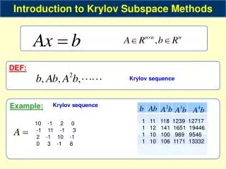
Introduction to Krylov Subspace Methods DEF: Krylov sequence Example: Krylov sequence 1 11 118 1239 12717 1 12 141 1651 19446 1 10 100 989 9546 1 10 106 1171 13332 10 -1 2 0 -1 11 -1 3 2 -1 10 -1 0 3 -1 8
Introduction to Krylov Subspace Methods DEF: Krylov subspace Example: Krylov subspace 10 -1 2 0 -1 11 -1 3 2 -1 10 -1 0 3 -1 8 DEF: Example: Krylov matrix
Introduction to Krylov Subspace Methods DEF: Example: Krylov matrix Remark:
WHY: Krylov Subspace Methods Example:Solve: DEF: Krylov matrix 10 -1 2 0 -1 11 -1 3 2 -1 10 -1 0 3 -1 8 >> A=[10 -1 2 0; -1 11 -1 3;2 -1 10 -1; 0 3 -1 8] >> poly(A) 1 -39 552 -3357 7395 Hence, Characteristic poly The key observation here is that the solution x to Ax = b is a linear combination of the vectors b and Ab,.. which make up the Krylov subspace the Cayley-Hamilton theorem a matrix satisfies its characteristic polynomial, p(A) = 0. That is, the solution to Ax = b has a natural representation as a member of a Krylov space, Multiplying with inv(A) & rearrange
Krylovsubspace Methods Krylov subspace others Conjugate Gradient GMRES MINRES
MATLAB commands Conjugate Gradient x = pcg(A, b, tol, maxit) MINRES x = minres(A, b, tol, maxit) GMRES x = gmres(A,b,[],tol,maxit)
Conjugate Gradient Method We want to solve the following linear system Conjugate Gradient Method
Conjugate Gradient Method Conjugate Gradient Method Example: Solve: 10 -1 2 0 -1 11 -1 3 2 -1 10 -1 0 3 -1 8 0 0.4716 0.9964 1.0015 1.0000 0 1.9651 1.9766 1.9833 2.0000 0 -0.8646 -0.9098 -1.0099 -1.0000 0 1.1791 1.0976 1.0197 1.0000 31.7 5.1503 1.0433 0.1929 0.0000