Example
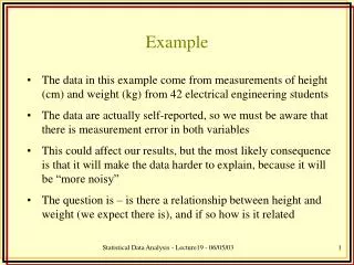
Example. The data in this example come from measurements of height (cm) and weight (kg) from 42 electrical engineering students The data are actually self-reported, so we must be aware that there is measurement error in both variables

Example
E N D
Presentation Transcript
Example • The data in this example come from measurements of height (cm) and weight (kg) from 42 electrical engineering students • The data are actually self-reported, so we must be aware that there is measurement error in both variables • This could affect our results, but the most likely consequence is that it will make the data harder to explain, because it will be “more noisy” • The question is – is there a relationship between height and weight (we expect there is), and if so how is it related Statistical Data Analysis - Lecture19 - 06/05/03
Plot the data There appears to be some evidence of a linear relationship between weight and height The relationship is positive => weight increases with height Statistical Data Analysis - Lecture19 - 06/05/03
Fit the model • We propose the following model • We fit the model in a very similar manner to that for ANOVA • fit<-lm(Weight~Height,data=heights) • To get some diagnostic plots (pred-res and norplot we type) • plot(fit) Statistical Data Analysis - Lecture19 - 06/05/03
Everything seems to be okay in the pred-res plot • There may be a slight funnel effect, but nothing significant Statistical Data Analysis - Lecture19 - 06/05/03
Our assumption of normality may be violated, but for the time being we will ignore this Statistical Data Analysis - Lecture19 - 06/05/03
> summary(fit) Call: lm(formula = Weight ~ Height, data = heights) Residuals: Min 1Q Median 3Q Max -16.310 -6.080 -2.714 5.574 20.021 Coefficients: Estimate Std. Error t value Pr(>|t|) (Intercept) -93.2313 26.0258 -3.582 0.000914 *** Height 0.9327 0.1492 6.252 2.09e-07 *** --- Signif. codes: 0 `***' 0.001 `**' 0.01 `*' 0.05 `.' 0.1 ` ' 1 Residual standard error: 8.851 on 40 degrees of freedom Multiple R-Squared: 0.4942, Adjusted R-squared: 0.4816 F-statistic: 39.09 on 1 and 40 degrees of freedom, p-value: 2.089e-007 Statistical Data Analysis - Lecture19 - 06/05/03
Influence • If one particular observation is a long way from the bulk of the data, i.e. if is large, then in will generally influence the fit • Outliers can cause many problems with statistical analyses • In regression, outliers have the potential to alter the fit • How? • Recall that the least squares procedure tries to minimise Statistical Data Analysis - Lecture19 - 06/05/03
The R2 for the black line is 0.8995 • When we drop the influential point from the analysis the R2 is 0.9805 • The lines may not look too different on the plot, but if we look at the regression tables we can see a vast difference Estimate Std.Err t-value Pr(>|t|) Intercept -49.1483 11.8924 -4.1327 1e-04 X 3.5482 0.1192 29.7659 0e+00 Intercept 7.7864 4.2126 1.8484 0.0676 X 2.9696 0.0423 70.1278 0.0000 Statistical Data Analysis - Lecture19 - 06/05/03
Outliers have the most influence when they are a long way from the mean of the x values and mean of the y values • You can think of the regression line as a plank on a fulcrum • The fulcrum is centered at the mean • If you place a heavy wieght near the fulcrum, the tilt of the plank will not change too much • However, if you place such a weight at the end on the plank then the tilt will change considerably • Points with high influence are also called high leverage points In this plot, although the point is a long way from the mean of the y values it is very close to the mean of the x values – consequently it will have a large residual, but will not be influential Statistical Data Analysis - Lecture19 - 06/05/03
Detecting influential observations • This can be hard to do • However, in general, if an observation has high influence then in will have a small residual • However, this in itself is not useful, we need to know how much each predictor played in giving the fitted value • Firstly, let us re-write our regression model in a more convenient form. Statistical Data Analysis - Lecture19 - 06/05/03
Matrix form of the regression model (not examinable) • Lety be a (n by 1) vector of responses, y= (y1,y2,…,yn)T • Let be a (2 by 1) vector of coefficients = (0, 1)T • Letbe a (n by 1) vector of errors, = (1, 2,…, n)T • And let Xbe a (n by 2) matrix with • Then we can rewrite our regression model as Statistical Data Analysis - Lecture19 - 06/05/03
Hat matrix • If we write our model in this form, then it is very simple to write down the least squares estimates of the slope and the intercept • Now if we multiply each side by X, then we get • The matrix His called the “hat matrix”, and this equation shows us that each fitted value is a (linear) combination of all the observed y values. Statistical Data Analysis - Lecture19 - 06/05/03
Hat matrix diagonals • More specifically • From this we can see that larger the hij value, the more influence yihas on the fitted value • In general, if hii (the ith diagonal element of the hat matrix) is large then the ith observation is influential • The values, hii for i = 1,…,n are called the hat matrix diagonals and are produced by most regression analysis packages (not Excel) Statistical Data Analysis - Lecture19 - 06/05/03
Small residual Large hat Large residual Large hat Small residual Small hat Large residual Small hat Leverage plots • The best way to use the hat matrix diagonals is in a leverage plot • A leverage plot puts the hat matrix diagonals on y-axis and the squared residuals on the x-axis • This plot can be divided into four quadrants: Statistical Data Analysis - Lecture19 - 06/05/03
Large hat matrix diagonal? • What do we mean by large? • It varies but there are a couple of rules of thumb • If k is the number of coefficients (excluding the intercept), then if hii > 2(k+1)/n a point might be worth an investigation. If hii > 3(k+1)/n a then this is large Statistical Data Analysis - Lecture19 - 06/05/03
Interpreting leverage plots • How do we interpret this plot? • If points are in the lower left quadrant, (small residual, small hat matrix diagonal) then we can ignore them • If they in the upper left (small residual, large hat matrix diagonal) we might consider these points influential and drop them from the regression • If they’re in the lower right corner (large residual, small hat matrix diagonal), then they’re not influential, but they will put unnecessary noise into the model – i.e. they don’t affect the fit, but they do affect the significance of the fit • If they’re in the upper right corner(large residual, large hat matrix diagonal) we’re in trouble! Statistical Data Analysis - Lecture19 - 06/05/03
Example • The data in the following example comes from ultrasound measurements on 40 babies. The variables are bi-parietal diameter (BPD) a measure of brain size in mm, and birth weight (BW) in grams. • The first thing we should do is? • We have two continuous variables relating to the same individual • Therefore a scatterplot is the most appropriate • We hope to see what trend (if any) exists in the data set Statistical Data Analysis - Lecture19 - 06/05/03
The relationship between BW and BPD looks approximately linear, therefore we propose a regression model Statistical Data Analysis - Lecture19 - 06/05/03
Fitting the model • We assume that BW and BPD are in a data frame called ‘babies’. We type • fit<-lm(BW~BPD,data=babies) • plot(fit) Statistical Data Analysis - Lecture19 - 06/05/03
The pred-res plot shows the residuals to be in a homogeneous band around zero • There is slight evidence that the residuals increase with the predictors • The norplot is approximately straight • There are a couple of residuals that are perhaps too large • There is some “bunching” in the plot Statistical Data Analysis - Lecture19 - 06/05/03
Constructing a leverage plot • We can ask R to give us the hat matrix diagonals for us as well as the residuals res<-resid(fit) hats<-lm.influence(fit)$hat • To construct the leverage plot we need the squared residuals • We make a new variable ressq ressq<-res^2 • We now plot the hats vs. ressq plot(ressq,hats) Statistical Data Analysis - Lecture19 - 06/05/03
We have one coefficient in this model (besides the intercept), so k = 1 and n = 40 observations, so 3(k+1)/n = 3*2/40 = 3/20=0.15 • Looking at our plot we can see there is one point that is larger than this bound • We find this is point 23 by the R statement: (1:40)[hats>0.15] Statistical Data Analysis - Lecture19 - 06/05/03
If we go back to the original data, we can see that point 23 is a “low birth weight” baby • This point has high leverage, because it is “anchoring” the regression line • What happens if we leave it out? Statistical Data Analysis - Lecture19 - 06/05/03
Regression Analysis (before deletion of pt 23) Call: lm(formula = BW ~ BPD, data = babies) Residuals: Min 1Q Median 3Q Max -287.72 -132.50 28.93 102.50 345.61 Coefficients: Estimate Std. Error t value Pr(>|t|) (Intercept) -2109.473 232.063 -9.09 4.52e-11 *** BPD 45.418 3.065 14.82 < 2e-16 *** --- Signif. codes: 0 `***' 0.001 `**' 0.01 `*' 0.05 `.' 0.1 ` ' 1 Residual standard error: 158.1 on 38 degrees of freedom Multiple R-Squared: 0.8525, Adjusted R-squared: 0.8486 F-statistic: 219.6 on 1 and 38 degrees of freedom, p-value: 0 Statistical Data Analysis - Lecture19 - 06/05/03
Call: lm(formula = BW ~ BPD, data = babies, subset = -23) Residuals: Min 1Q Median 3Q Max -285.75 -137.38 14.09 111.16 347.62 Coefficients: Estimate Std. Error t value Pr(>|t|) (Intercept) -2208.988 254.803 -8.669 1.93e-10 *** BPD 46.685 3.345 13.956 2.22e-16 *** --- Signif. codes: 0 `***' 0.001 `**' 0.01 `*' 0.05 `.' 0.1 ` ' 1 Residual standard error: 158.3 on 37 degrees of freedom Multiple R-Squared: 0.8404, Adjusted R-squared: 0.8361 F-statistic: 194.8 on 1 and 37 degrees of freedom, p-value: 2.22e-016 Statistical Data Analysis - Lecture19 - 06/05/03
Removing influential points • Rarely successful • Especially when we have the anchoring situation as with this data • What usually happens is that as you delete one “influential” point another becomes influential • So what should we do? • Only remove points if it substantially improves model fit • I.e. if the adj-R2 increases. • If the coefficients change • If the significance changes • Always record which points you removed and why Statistical Data Analysis - Lecture19 - 06/05/03

