Polynomial Functions and Models
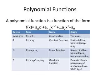
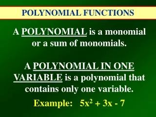
Polynomial Functions and Models. Lesson 4.2. Review. General polynomial formula a 0 , a 1 , … ,a n are constant coefficients n is the degree of the polynomial Standard form is for descending powers of x a n x n is said to be the “leading term”. •. •.

Polynomial Functions and Models
E N D
Presentation Transcript
Polynomial Functions and Models Lesson 4.2
Review • General polynomial formula • a0, a1, … ,an are constant coefficients • n is the degree of the polynomial • Standard form is for descending powers of x • anxn is said to be the “leading term”
• • Turning Points and Local Extrema • Turning point • A point (x, y) on the graph • Located where graph changes • from increasing • to decreasing • (or vice versa)
Family of Polynomials • Constant polynomial functions • f(x) = a • Linear polynomial functions • f(x) = m x + b • Quadratic polynomial functions • f(x) = a x2 + b x + c
Family of Polynomials • Cubic polynomial functions • f(x) = a x3 + b x2 + c x + d • Degree 3 polynomial • Quartic polynomial functions • f(x) = a x4 + b x3 + c x2+ d x + e • Degree 4 polynomial
Compare Long Run Behavior Consider the following graphs: • f(x) = x4 - 4x3 + 16x - 16 • g(x) = x4 - 4x3 - 4x2 +16x • h(x) = x4 + x3 - 8x2 - 12x • Graph these on the window -8 < x < 8 and 0 < y < 4000 • Decide how these functions are alike or different, based on the view of this graph
Compare Long Run Behavior • From this view, they appear very similar
Contrast Short Run Behavior • Now Change the window to be-5 < x < 5 and -35 < y < 15 • How do the functions appear to be different from this view?
Contrast Short Run Behavior Differences? • Real zeros • Local extrema • Complexzeros • Note: The standard form of the polynomials does not give any clues as to this short run behavior of the polynomials:
Assignment • Lesson 4.2A • Page 270 • Exercises 1 – 38 odd
Piecewise Defined Functions • Consider • Sketch graph • Use calculator to display • Consider if f(x) is continuous
Linear Regression • Used in section previous lessons to find equation for a line of best fit • Other types of regression are available
Polynomial Regression • Consider the lobster catch (in millions of lbs.) in the last 30 some years • Enter into Data Matrix
Viewing the Data Points • Specify the plot F2, • X's from C1, Y's from C2 • View thegraph • Check Y= screen, use Zoom-Data
Polynomial Regression • Try for 4th degreepolynomial
Other Technology Tools • Excel will also do regression • Plot data as (x,y) ordered pairs • Right click on data series • Choose Add Trend Line
Other Technology Tools • Use dialog box to specify regression Try Others
Try It Out … • An object is lifted rapidly into the air and then released. The table shows the height at t seconds after the start of the experiment • Use your calculator to plot the data • At what time was the object released? • What part of the time interval could be represented by a linear function? Find that function. • Find a modeling function for the non linear portion.
Assignment • Lesson 4.2B • Page 273 • Exercises 41 – 89 EOO