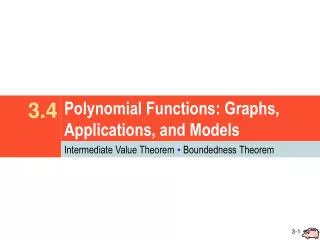
Polynomial Functions: Graphs, Applications, and Models

1. Objectives Students will learn how to: Graph functions (x) = axn Graph General Polynomial Functions Find Turning Points and End Behavior Intermediate Value Theorems Approximate Real Zeros Using Graphing Calculator Use Graphing Calculator to Determine Polynomial Models and Curve Fitting Polynomial Functions: Graphs, Applications, and Models

2. Example 1 GRAPHING FUNCTIONS OF THE FORM (x) = axn Graph the function. a. Solution Choose several values for x, and find the corresponding values of (x), or y.

3. Example 1 GRAPHING FUNCTIONS OF THE FORM (x) = axn Graph the function. b. Solution The graphs of (x) = x3 and g(x) = x5are both symmetric with respect to the origin.

4. Example 1 GRAPHING FUNCTIONS OF THE FORM (x) = axn Graph the function. c. Solution The graphs of (x) = x3 and g(x) = x5are both symmetric with respect to the origin.

5. Graphs of General Polynomial Functions As with quadratic functions, the absolute value of a in (x) = axn determines the width of the graph. When a> 1, the graph is stretched vertically, making it narrower, while when 0 < a < 1, the graph is shrunk or compressed vertically, so the graph is broader. The graph of (x) = –axnis reflected across the x-axis compared to the graph of (x) = axn.

6. Graphs of General Polynomial Functions Compared with the graph of the graph of is translated (shifted) k units up if k > 0 andkunits down if k < 0. Also, when compared with the graph of the graph of (x) = a(x – h)nis translated h units to the right if h > 0 and hunits to the left if h < 0. The graph of shows a combination of these translations. The effects here are the same as those we saw earlier with quadratic functions.

7. Example 2 EXAMINING VERTICAL AND HORIZONTAL TRANSLATIONS Graph the function. a. Solution The graph will be the same as that of (x) = x5, but translated 2 units down.

8. Example 2 EXAMINING VERTICAL AND HORIZONTAL TRANSLATIONS Graph the function. b. Solution In (x) = (x + 1)6, function  has a graph like that of (x) = x6, but since x + 1 = x– (–1), it is translated 1 unit to the left.

9. Example 2 EXAMINING VERTICAL AND HORIZONTAL TRANSLATIONS Graph the function. c. Solution The negative sign in –2 causes the graph of the function to be reflected across the x-axis when compared with the graph of (x) = x3. Because –2> 1, the graph is stretched vertically as compared to the graph of (x) = x3. It is also translated 1 unit to the right and 3 units up.

10. Unless otherwise restricted, the domain of a polynomial function is the set of all real numbers. Polynomial functions are smooth, continuous curves on the interval (–, ). The range of a polynomial function of odd degree is also the set of all real numbers. Typical graphs of polynomial functions of odd degree are shown in next slide. These graphs suggest that for every polynomial function  of odd degree there is at least one real value of x that makes (x) = 0. The real zeros are the x-intercepts of the graph.

11. Odd Degree

12. A polynomial function of even degree has a range of the form (–, k] or [k, ) for some real number k. Here are two typical graphs of polynomial functions of even degree. Even Degree

13. Recall that a zero c of a polynomial function has as multiplicity the exponent of the factor x – c. Determining the multiplicity of a zero aids in sketching the graph near that zero. If the zero has multiplicity one, the graph crosses the x-axis at the corresponding x-intercept as seen here.

14. If the zero has even multiplicity, the graph is tangent to the x-axis at the corresponding x-intercept (that is, it touches but does not cross the x-axis there).

15. If the zero has odd multiplicity greater than one, the graph crosses the x-axisand is tangent to the x-axis at the corresponding x-intercept. This causes a change in concavity, or shape, at the x-intercept and the graph wiggles there.

16. Turning Points and End Behavior The previous graphs show that polynomial functions often have turning points where the function changes from increasing to decreasing or from decreasing to increasing.

17. Turning Points A polynomial function of degree n has at most n – 1 turning points, with at least one turning point between each pair of successive zeros.

18. End Behavior The end behavior of a polynomial graph is determined by the dominating term, that is, the term of greatest degree. A polynomial of the form has the same end behavior as .

19. End Behavior For instance, has the same end behavior as . It is large and positive for large positive values of x and large and negative for negative values of x with large absolute value.

20. End Behavior The arrows at the ends of the graph look like those of the graph shown here; the right arrow points up and the left arrow points down. The graph shows that as x takes on larger and larger positive values, y does also. This is symbolized as read “as x approaches infinity, y approaches infinity.”

21. End Behavior For the same graph, as x takes on negative values of larger and larger absolute value, y does also: as

22. End Behavior For this graph, we have as and as

23. End Behavior of Polynomials • Suppose that axn is the dominating term of a polynomial function  of odd degree. • If a > 0, then as and as • Therefore, the end behavior of the graph is of the type that looks like the figure shown here. • We symbolize it as .

24. End Behavior of Polynomials Suppose that axn is the dominating term of a polynomial function  of odd degree. 2. If a < 0, then as and as Therefore, the end behavior of the graph looks like the graph shown here. We symbolize it as .

25. End Behavior of Polynomials • Suppose that axn is the dominating term of a polynomial function of even degree. • If a > 0, then as • Therefore, the end behavior of the • graph looks like the graph shown here. • We symbolize it as .

26. End Behavior of Polynomials Suppose that is the dominating term of a polynomial function  of even degree. 2. If a < 0, then as Therefore, the end behavior of the graph looks like the graph shown here. We symbolize it as .

27. Example 3 DETERMINING END BEHAVIOR GIVEN THE DEFINING POLYNOMIAL Match each function with its graph. A. B. C. D. Solution Because  is of even degree with positive leading coefficient, its graph is C.

28. Example 3 DETERMINING END BEHAVIOR GIVEN THE DEFINING POLYNOMIAL Match each function with its graph. A. B. C. D. Solution Because g is of even degree with negative leading coefficient, its graph is A.

29. Example 3 DETERMINING END BEHAVIOR GIVEN THE DEFINING POLYNOMIAL Match each function with its graph. A. B. C. D. Solution Because function h has odd degree and the dominating term is positive, its graph is in B.

30. Example 3 DETERMINING END BEHAVIOR GIVEN THE DEFINING POLYNOMIAL Match each function with its graph. A. B. C. D. Solution Because function k has odd degree and a negative dominating term, its graph is in D.

31. Graphing Techniques We have discussed several characteristics of the graphs of polynomial functions that are useful for graphing the function by hand. A comprehensive graph of a polynomial function will show the following characteristics: 1. all x-intercepts (zeros) 2. the y-intercept 3. the sign of (x) within the intervals formed by the x-intercepts, and all turning points 4. enough of the domain to show the end behavior. In Example 4, we sketch the graph of a polynomial function by hand. While there are several ways to approach this, here are some guidelines.

32. Graphing a Polynomial Function Let be a polynomial function of degree n. To sketch its graph, follow these steps. Step 1 Find the real zeros of . Plot them as x-intercepts. Step 2 Find (0). Plot this as the y-intercept.

33. Graphing a Polynomial Function Step 3 Use test points within the intervals formed by the x-intercepts to determine the sign of (x) in the interval. This will determine whether the graph is above or below the x-axis in that interval.

34. Graphing a Polynomial Function Use end behavior, whether the graph crosses, bounces on, or wiggles through the x-axis at the x-intercepts, and selected points as necessary to complete the graph.

35. Objectives Students will learn how to: Synthetic Division Solve Equations of Higher Order Than Quadratics by Factoring Use Synthetic Division to Divide Polynomials Evaluate Polynomial Functions Using the Remainder Theorem (synthetic substitution) Test Potential Zeros (Roots, Solutions)

36. Solving Higher Degree Equations by Factoring The equation x3 + 8 = 0 that follows is called a cubic equation because of the degree 3 term. Some higher-degree equations can be solved using factoring and/or the quadratic formula.

37. SOLVING A CUBIC EQUATION Solve Solution Factor as a sum of cubes. or Zero-factor property or Quadratic formula; a = 1, b = –2, c = 4

38. SOLVING A CUBIC EQUATION Solve Solution Simplify. Simplify the radical. Factor out 2 in the numerator.

39. SOLVING A CUBIC EQUATION Solve Solution Lowest terms

40. SOLVING A CUBIC EQUATION Solve Factor out common factor Factor completely if possible or use other methods. Set each factor equal to zero and solve

41. SOLVING A CUBIC EQUATION Solution set x={0,8,-6}

42. If a polynomial is not easily factored than we must use division to determine the solutions Division Algorithm Let (x) and g(x) be polynomials with g(x) of lower degree than (x) and g(x) of degree one or more. There exists unique polynomials q(x) and r(x) such that where either r(x) = 0 or the degree of r(x) is less than the degree of g(x).

43. Synthetic Division Synthetic division is a shortcut method of performing long division with polynomials. It is used only when a polynomial is divided by a first-degree binomial of the form x – k, where the coefficient of x is 1.

44. Traditional Division Divide by Remainder Quotient

45. Synthetic Division Remainder Quotient CautionTo avoid errors, use 0 as the coefficient for any missing terms, including a missing constant, when setting up the division.

46. Example 1 USING SYNTHETIC DIVISION Use synthetic division to divide Solution Express x + 2 in the form x – k by writing it as x– (–2). Use this and the coefficients of the polynomial to obtain x + 2 leads to–2 Coefficients

47. Example 1 USING SYNTHETIC DIVISION Use synthetic division to divide Solution Bring down the 5, and multiply: –2(5) = –10

48. Example 1 USING SYNTHETIC DIVISION Use synthetic division to divide Solution Add –6 and –10 to obtain –16. Multiply –2(–16) = 32.

49. Example 1 USING SYNTHETIC DIVISION Use synthetic division to divide Solution Add –28 and 32 to obtain 4. Finally, –2(4) = – 8. Add columns. Watch your signs.

50. Example 1 USING SYNTHETIC DIVISION Use synthetic division to divide Solution Add –2 and –8 to obtain –10. Remainder Quotient