Download
1 / 17
240 likes | 368 Views
Learn about cubic functions, how to plot graphs, find roots, interpret transformations, and sketch functions. Understand the behavior of curves and identify turning points. Explore multiple zeros and their impact on graphs.

E N D
Cubic functions parent function: f(x) = x3 none vertical asymptote: none horizontal asymptote: domain: (– ∞, ∞) (– ∞, ∞) range: roots: x = 0
Using a table of values Plot the graph of y = x3 – 7x + 2 for values of x between –3 and 3. Complete the table of values. Plot the points from the table on the graph paper. Join the points together with a smooth curve.
General form general cubic function: f(x)= ax3 + bx2 + cx + d where a ≠ 0 When the coefficient of x3 is positive the shape is: none vertical asymptote: none horizontal asymptote: or domain: (– ∞, ∞) When the coefficient of x3 is negative the shape is: (– ∞, ∞) range: or
Sketching graphs What can we find to help us sketch the graph of a function? 1) find the point where the curve intersects the y-axis by evaluating f(0) 2) find any points where the curve intersects the x-axis by solvingf(x) = 0 3) predict the behavior of y when x is very large and positive 4) predict the behavior of y when x is very large and negative 5) estimate turning points. When a cubic function is written in factored form y = a(x–p)(x–q)(x–r), where does it intersect the x-axis? The graph intersects the x-axis at the points (p, 0), (q, 0) and (r, 0). p, q and r are the roots of the cubic function.
Sketching cubic graphs (1) Sketch the graph of y = x3 + 2x2 – 3x. 1) find y-intercept: evaluate f(0): f(0) = 03 + 2(0)2 – 3(0) f(0) = 0 The curve passes through the point (0, 0). 2) find x-intercepts: setf(x) = 0: x3 + 2x2 – 3x = 0 GCF: x(x2 + 2x – 3) = 0 by grouping: x(x + 3)(x – 1) = 0 zero product: x = 0, x = –3 or x = 1 The curve also passes through the points (–3, 0) and (1, 0).
Sketching cubic graphs (2) Sketch the graph of y = x3 + 2x2 – 3x. 3) as x→ ∞, y → ∞ 4) as x→ –∞, y → –∞ 5) estimate turning points: since cubic: at most 2 turning points x-value: between –3 and 0 and 0 and 1 estimate y: f(–1.5) = 5.625 f(0.5) = –0.875
Multiple zeros Give the multiplicity of each zero in the functiony = (x + 2)(x + 1)2(x – 1)3. x = –2 has multiplicity 1 x = –1 has multiplicity 2 x = 1 has multiplicity 3. Now describe the behavior of the graph at each zero. Do you notice a pattern? The behavior of a graph at a zero of multiplicity n resembles the behavior of y = xn at zero.
Multiple zeros example Sketch the graph of y = (x + 1)2(x – 1). 1) find y-intercept: evaluate f(0): f(0) = –1 The curve passes through (0, –1). 2) find x-intercepts: setf(x) = 0: (x + 1)2(x – 1) = 0 zero product property: x = –1 or x = 1 The curve passes through (–1, 0) and (1, 0). 3) as x→ ∞, y → ∞ 4) as x→ –∞, y → –∞ 5) estimate turning points: Since x = –1 is a zero of multiplicity 2, the behavior of the graph at –1 is similar to quadratic, so that is a relative maxima.
Sketching quartic graphs (1) Sketch the graph of y = x4 – 5x2 + 4. 1) find y-intercept: evaluate f(0): f(0) = 04 – 5(0)2 + 4 f(0) = 4 The curve passes through the point (0, 4). 2) find x-intercepts: setf(x) = 0: x4 – 5x2 + 4= 0 (x2)2 – 5(x2) + 4= 0 (x2 – 1)(x2 – 4) = 0 difference of squares: (x + 1)(x – 1)(x + 2)(x – 2) = 0 zero product property: x = ±1 and x = ±2 The curve also passes through the points (–2, 0), (–1, 0), (1, 0) and (2, 0).
Sketching quartic graphs (2) Sketch the graph of y = x4 – 5x2 + 4. 3) as x→ ∞, y → ∞ 4) as x→ –∞, y → ∞ 5) estimate turning points: since quartic: at most 3 turning points x-value: between –1 and 1, between –2 and –1, and between 1 and 2 estimate y: f(0) = 4 f(–1.5) = –2.1875 f(1.5) = –2.1875