Continuous Random Variables
Continuous Random Variables. Continuous Random Variable. A continuous random variable is one for which the outcome can be any value in an interval of the real number line. Usually a measurement. Examples Let Y = length in mm Let Y = time in seconds Let Y = temperature in ºC.

Continuous Random Variables
E N D
Presentation Transcript
Continuous Random Variable • A continuous random variable is one for which the outcome can be any value in an interval of the real number line. • Usually a measurement. • Examples • Let Y = length in mm • Let Y = time in seconds • Let Y = temperature in ºC L. Wang, Department of Statistics University of South Carolina; Slide 2
Continuous Random Variable • We don’t calculate P(Y = y), we calculate P(a < Y < b), where a and b are real numbers. • For a continuous random variable P(Y = y) = 0. L. Wang, Department of Statistics University of South Carolina; Slide 3
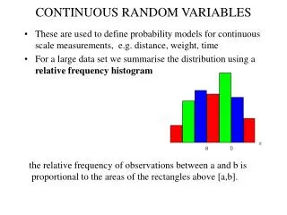
Continuous Random Variables • The probability density function (pdf) when plotted against the possible values of Y forms a curve. The area under an interval of the curve is equal to the probability that Y is in that interval. 0.40 f(y) a b Y L. Wang, Department of Statistics University of South Carolina; Slide 4
The entire area under a probability density curve for a continuous random variable • Is always greater than 1. • Is always less than 1. • Is always equal to 1. • Is undeterminable. L. Wang, Department of Statistics University of South Carolina; Slide 5
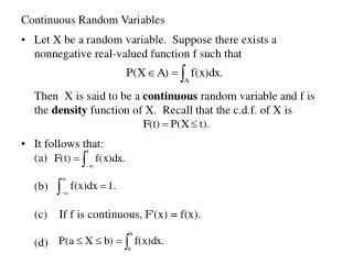
Properties of a Probability Density Function (pdf) • f(y) > 0 for all possible intervals of y. • If y0 is a specific value of interest, then the cumulative distribution function (cdf) is • If y1 and y2 are specific values of interest, then L. Wang, Department of Statistics University of South Carolina; Slide 6
Grams of lead per liter of gasoline has the probability density function: f(y) = 12.5y - 1.25for 0.1 < y < 0.5What is the probability that the next liter of gasoline has less than 0.3 grams of lead? L. Wang, Department of Statistics University of South Carolina; Slide 7
Suppose a random variable Y has the following probability density function: f(y) = y if 0<y<1 2-y if 1 < y<2 0 if 2 < y.Find the complete form of the cumulative distribution function F(y) for any real value y. L. Wang, Department of Statistics University of South Carolina; Slide 8
Expected Value for a Continuous Random Variable • Recall Expected Value for a discrete random variable: • Expected value for a continuous random variable: L. Wang, Department of Statistics University of South Carolina; Slide 9
Variance for Continuous Random Variable Recall: Variance for a discrete random variable: Variance for a continuous random variable: L. Wang, Department of Statistics University of South Carolina; Slide 10
Difference between Discreteand continuous random variables • Possible values that can be assumed • Probability distribution function • Cumulative distribution function • Expected value • Variance L. Wang, Department of Statistics University of South Carolina; Slide 11
Times Between Industrial Accidents • The times between accidents for a 10-year period at a DuPont facility can be modeled by the exponential distribution. where λ is the accident rate (the expected number of accidents per day in this case) L. Wang, Department of Statistics University of South Carolina; Slide 12
Example of time between accidents Let Y = the number of days between two accidents. Time 12 days 35 days 5 days ● ● ● ● ● Accident Accident Accident #1 #2 #3 L. Wang, Department of Statistics University of South Carolina; Slide 13
Times Between Industrial Accidents • Suppose in a 1000 day period there were 50 accidents. λ = 50/1000 = 0.05 accidents per day or 1/λ = 1000/50 = 20 days between accidents L. Wang, Department of Statistics University of South Carolina; Slide 14
What is the probability that this facility will go less than 10 days between the next two accidents? ? f(y) = 0.05e-0.05y L. Wang, Department of Statistics University of South Carolina; Slide 15
? Recall: L. Wang, Department of Statistics University of South Carolina; Slide 16
In General… L. Wang, Department of Statistics University of South Carolina; Slide 17
Exponential Distribution L. Wang, Department of Statistics University of South Carolina; Slide 18
If the time to failure for an electrical component follows an exponential distribution with a mean time to failure of 1000 hours, what is the probability that a randomly chosen component will fail before 750 hours? Hint: λ is the failure rate (expected number of failures per hour). L. Wang, Department of Statistics University of South Carolina; Slide 19
Mean and Variance for an Exponential Random Variable Note: Mean = Standard Deviation L. Wang, Department of Statistics University of South Carolina; Slide 20
The time between accidents at a factory follows an exponential distribution with a historical average of 1 accident every 900 days. What is the probability that that there will be more than 1200 days between the next two accidents? L. Wang, Department of Statistics University of South Carolina; Slide 21
If the time between accidents follows an exponential distribution with a mean of 900 days, what is the probability that there will be less than 900 days between the next two accidents? L. Wang, Department of Statistics University of South Carolina; Slide 22
Relationship between Exponential & Poisson Distributions • Recall that the Poisson distribution is used to compute the probability of a specific number of events occurring in a particular interval of time or space. • Instead of the number of events being the random variable, consider the time or space between events as the random variable. L. Wang, Department of Statistics University of South Carolina; Slide 23
Relationship between Exponential & Poisson Exponential distribution models time (or space) between Poisson events. TIME L. Wang, Department of Statistics University of South Carolina; Slide 24
Exponential or Poisson Distribution? • We model the number of industrial accidents occurring in one year. • We model the length of time between two industrial accidents (assuming an accident occurring is a Poisson event). • We model the time between radioactive particles passing by a counter (assuming a particle passing by is a Poisson event). • We model the number of radioactive particles passing by a counter in one hour L. Wang, Department of Statistics University of South Carolina; Slide 25
Recall: For a Poisson Distribution y = 0,1,2,… where λ is the mean number of events per base unit of time or space and t is the number of base units inspected. The probability that no events occur in a span of time (or space) is: L. Wang, Department of Statistics University of South Carolina; Slide 26
Now let T = the time (or space) until the next Poisson event. In other words, the probability that the length of time (or space) until the next event is greater than some given time (or space), t, is the same as the probability that no events will occur in time (or space) t. L. Wang, Department of Statistics University of South Carolina; Slide 27
Radioactive Particles • The arrival of radioactive particles at a counter are Poisson events. So the number of particles in an interval of time follows a Poisson distribution. Suppose we average 2 particles per millisecond. • What is the probability that no particles will pass the counter in the next 3 milliseconds? • What is the probability that more than 3 millisecond will elapse before the next particle passes? L. Wang, Department of Statistics University of South Carolina; Slide 28
Machine Failures • If the number of machine failures in a given interval of time follows a Poisson distribution with an average of 1 failure per 1000 hours, what is the probability that there will be no failures during the next 2000 hours? • What is the probability that the time until the next failure is more than 2000 hours? L. Wang, Department of Statistics University of South Carolina; Slide 29
Number of failures in an interval of time follows a Poisson distribution. If the mean time to failure is 1000 hours, what is the probability that more than 2500 hours will pass before the next failure occurs? • e-4 • 1 – e-4 • e-2.5 • 1 – e-2.5 L. Wang, Department of Statistics University of South Carolina; Slide 30
If ten of these components are used in different devices that run independently, what is the probability that at least one will still be operating at 2500 hours?What about he probability that exact 3 of them will be still operating after 2500 hours? Challenging questions L. Wang, Department of Statistics University of South Carolina; Slide 31
Normal Distribution f(y) = E[Y] = μ and Var[Y] = σ2 f(y) y L. Wang, Department of Statistics University of South Carolina; Slide 32
Normal Distribution • Characteristics • Bell-shaped curve • - < y< + • μ determines distribution location and is the highest point on curve • Curve is symmetric about μ • σ determines distribution spread • Curve has its points of inflection at μ + σ L. Wang, Department of Statistics University of South Carolina; Slide 33
Normal Distribution σ σ σ σ σ μ L. Wang, Department of Statistics University of South Carolina; Slide 34
Normal Distribution N(μ = 5, σ = 1) N(μ = 0, σ = 1) f(y) y L. Wang, Department of Statistics University of South Carolina; Slide 35
Normal Distribution N(μ = 0,σ = 0.5) f(y) N(μ = 0,σ = 1) y L. Wang, Department of Statistics University of South Carolina; Slide 36
Normal Distribution N(μ = 5, σ = 0.5) N(μ = 0, σ = 1) f(y) y L. Wang, Department of Statistics University of South Carolina; Slide 37
68-95-99.7 Rule 0.997 0.95 0.68 µ µ-3σ µ-2σ µ-1σ µ+1σ µ+2σ µ+3σ μ + 1σ covers approximately 68% μ + 2σ covers approximately 95% μ + 3σ covers approximately99.7% L. Wang, Department of Statistics University of South Carolina; Slide 38
Earthquakes in a California Town Since 1900, the magnitude of earthquakes that measure 0.1 or higher on the Richter Scale in a certain location in California is distributed approximately normally, with μ = 6.2 and σ = 0.5, according to data obtained from the United States Geological Survey. L. Wang, Department of Statistics University of South Carolina; Slide 39
Earthquake Richter Scale Readings 34% 34% 2.5% 2.5% 13.5% 13.5% 5.2 5.7 6.2 6.7 7.2 68% 57 159 95% L. Wang, Department of Statistics University of South Carolina; Slide 40
Approximately what percent of the earthquakes are above 5.7 on the Richter Scale? 34% 34% 2.5% 2.5% 13.5% 13.5% 5.2 5.7 6.2 6.7 7.2 68% 95% L. Wang, Department of Statistics University of South Carolina; Slide 41
The highest an earthquake can read and still be in the lowest 2.5% is _. 34% 34% 2.5% 2.5% 13.5% 13.5% 5.2 5.7 6.2 6.7 7.2 68% 95% L. Wang, Department of Statistics University of South Carolina; Slide 42
The approximate probability an earthquake is above 6.7 is ______. 34% 34% 2.5% 2.5% 13.5% 13.5% 5.2 5.7 6.2 6.7 7.2 68% 95% L. Wang, Department of Statistics University of South Carolina; Slide 43
Standard Normal Distribution • Standard normal distribution is the normal distribution that has a mean of 0 and standard deviation of 1. N(µ = 0, σ = 1) L. Wang, Department of Statistics University of South Carolina; Slide 44
Z is Traditionally used as the Symbol for a Standard Normal Random Variable Z Y 4.7 5.2 5.7 6.2 6.7 7.2 7.7 L. Wang, Department of Statistics University of South Carolina; Slide 45
Normal Standard Normal Any normally distributed random variable can be converted to standard normal using the following formula: We can compare observations from two different normal distributions by converting the observations to standard normal and comparing the standardized observations. L. Wang, Department of Statistics University of South Carolina; Slide 46
What is the standard normal value (or Z value) for a Richter reading of 6.5?Recall Y ~ N(µ=6.2, σ=0.5) L. Wang, Department of Statistics University of South Carolina; Slide 47
Example • Consider two towns in California. The distributions of the Richter readings over 0.1 in the two towns are: Town 1: X ~ N(µ = 6.2, σ = 0.5) Town 2: Y ~ N(µ = 6.2, σ = 1). - What is the probability that Town 1 has an earthquake over 7 (on the Richter scale)? - What is the probability that Town 2 has an earthquake over 7? L. Wang, Department of Statistics University of South Carolina; Slide 48
Town 1 Town 2 Town 1: Town 2: 0.212 0.055 Z Z X Y 4.7 5.2 5.7 6.2 6.7 7.2 7.7 3.2 4.2 5.2 6.2 7.2 8.2 9.2 L. Wang, Department of Statistics University of South Carolina; Slide 49
Standard Normal 0.10 0.10 0.05 0.05 0.025 0.025 0.01 0.01 0.005 0.005 1.645 -1.645 2.326 -2.326 1.282 1.96 2.576 -2.576 -1.96 -1.282 L. Wang, Department of Statistics University of South Carolina; Slide 50

