Download
1 / 41
410 likes | 487 Views
NEW ANALYTIC APPROACHES TO THE CONSTRUCTION OF A SPHERICAL HARMONIC GEOPOTENTIAL MODEL. Sten Claessens and Will Featherstone Western Australian Centre for Geodesy Curtin University of Technology Perth, Australia. Dynamic Planet 2005, 25 August. Introduction.

E N D
NEW ANALYTIC APPROACHES TO THE CONSTRUCTION OF A SPHERICAL HARMONIC GEOPOTENTIAL MODEL Sten Claessens and Will Featherstone Western Australian Centre for Geodesy Curtin University of Technology Perth, Australia Dynamic Planet 2005, 25 August
Introduction COMPUTATION OF GEOPOTENTIAL COEFFICIENTSFROM GRAVITY ANOMALIES (Block-Diagonal) Least Squares estimation Numerical Quadrature based on analytic solutions
Introduction COMPUTATION OF GEOPOTENTIAL COEFFICIENTSFROM GRAVITY ANOMALIES (Block-Diagonal) Least Squares estimation prone to aliasing effects in higher degrees Numerical Quadrature based on analytic solutions
Introduction COMPUTATION OF GEOPOTENTIAL COEFFICIENTSFROM GRAVITY ANOMALIES • (Block-Diagonal) Least Squares estimation • prone to aliasing effects in higher degrees • Numerical Quadrature based on analytic solutions • Ellipsoidal harmonics conversion (Jekeli) • Weighted summation over spherically approximated coefficients
Analytic approaches (1/4) ellipsoid space domain
Analytic approaches (1/4) ellipsoid space domain SHS frequency domain solid harmonics
Analytic approaches (1/4) ellipsoid sphere space upward continuation domain SHS frequency domain solid harmonics
Analytic approaches (1/4) ellipsoid sphere space upward continuation domain SHS SHA frequency domain solid harmonics
Analytic approaches (1/4) ellipsoid sphere space upward continuation domain SHS SHA frequency domain solid harmonics
Analytic approaches (2/4) ellipsoid sphere space upward continuation domain SHS ellipsoidal integration SHA frequency domain solid harmonics
Analytic approaches (3/4) ellipsoid sphere space upward continuation domain SHA SHS ellipsoidal integration SHA frequency domain surface harmonics solid harmonics
Analytic approaches (3/4) ellipsoid sphere space upward continuation domain SHA SHS ellipsoidal integration SHA frequency coefficient transformation domain surface harmonics solid harmonics
Analytic approaches (4/4) COEFFICIENT TRANSFORMATION
Analytic approaches (4/4) COEFFICIENT TRANSFORMATION
Analytic approaches (4/4) COEFFICIENT TRANSFORMATION
Analytic approaches (4/4) COEFFICIENT TRANSFORMATION
Analytic approaches (4/4) COEFFICIENT TRANSFORMATION
Analytic approaches (4/4) COEFFICIENT TRANSFORMATION
Analytic approaches (4/4) COEFFICIENT TRANSFORMATION
Analytic approaches (4/4) COEFFICIENT TRANSFORMATION
Analytic approaches (4/4) COEFFICIENT TRANSFORMATION
Analytic approaches (4/4) COEFFICIENT TRANSFORMATION
Numerical comparison (1/3) Weights for zonal harmonics
Numerical comparison (1/3) Weights for zonal harmonics
Numerical comparison (1/3) Weights for zonal harmonics
Numerical comparison (1/3) Weights for zonal harmonics
Numerical comparison (1/3) Weights for zonal harmonics
Numerical comparison (3/3) Geoid height errors – spherical approximation Min: -5.84m difference in geoid height (m) (n=20-360) Max: 7.85m
Numerical comparison (3/3) Geoid height errors – Cruz/Sjöberg Min: -3.19m difference in geoid height (m) (n=20-360) Max: 2.60m
Numerical comparison (3/3) Geoid height errors – Petrovskaya et al. Min: -0.65m difference in geoid height (m) (n=20-360) Max: 0.81m
Numerical comparison (3/3) Geoid height errors – ellipsoidal integration Min: -0.065m difference in geoid height (m) (n=20-360) Max: 0.069m
Numerical comparison (3/3) Geoid height errors – coefficient transformation Min: -0.0021m difference in geoid height (m) (n=20-360) Max: 0.0026m
Numerical comparison (3/3) Geoid height errors – Jekeli Min: -0.00018m difference in geoid height (m) (n=20-360) Max: 0.00016m
Summary and conclusions • Three methods for the computation of geopotential coefficients have been derived rigorously • The accuracy of these methods is significantly higher than existing methods • Numerical tests have shown that the Coefficient Transformation approach performs best, improving on Jekeli’s approach for coefficients of low order m
Acknowledgements Thanks are extended to Dr. Simon Holmes of Raytheon ITSS, USA, for providing test data and Jekeli’s solution