Download
1 / 22
230 likes | 391 Views
A Practical Analytic Model for Daylight. A. J. Preetham, Peter Shirley, Brian Smits SIGGRAPH ’99 Presentation by Jesse Hall. Introduction. Outdoor scenes are becoming more feasible and common Most light comes from sun and sky Distances make atmosphere visible. Example.

E N D
A Practical Analytic Modelfor Daylight A. J. Preetham, Peter Shirley, Brian Smits SIGGRAPH ’99 Presentation by Jesse Hall
Introduction • Outdoor scenes are becoming more feasible and common • Most light comes from sun and sky • Distances make atmosphere visible
Example Important in photographs, paintings
Goals • Accurate formulas for sun and sky color, aerial perspective effects • Simple, intuitive parameters • Location, direction, date, time of day, conditions… • Computationally efficient
Background • Sky color and aerial perspective are caused by atmospheric scattering of light (Minneart 1954) • Primary and secondary scattering most important
Scattering: Air Molecules • Most important scattering due to air molecules • Molecules smaller than wavelength: Rayleigh scattering • Wavelength-dependent scattering gives sky overall blue color • Also causes yellow/orange sun, sunsets
Scattering: Haze • Light also scattered by ‘haze’ particles (smoke, dust, smog) • Haze particles larger than wavelength: Mie scattering, wavelength independent • Usually approximated with turbidity parameter: T = (tm+th)/tm
Previous Work: Sky Color • Explicit modeling • Measured data • CIE IDMP, Ineichen 1994 • Simulation • Klassen 1987, Kaneda 1992, Nishita 1996 • Analytic • CIE formula 1994, Perez 1993
Previous Work:Aerial Perspective • Explicit modeling • Simulation • Ebert et al. 1998 • Analytic model for fog • Kaneda 1991 • Simple non-directional models • Ward-Larson 1998 (Radiance)
Sunlight & Skylight • Input: sun position, turbidity • Output: spectral radiance • Sun position calculated from latitude, longitude, time, date • Haze density based on turbidity and measured data
Sunlight • Look up spectral radiance outside atmosphere in table • Calculate attenuation from different particles using constants given in Iqbal 1983 • Multiply extra-terrestrial spectral radiance by all attenuation coefficients to get direct spectral radiance
Skylight: Model • Use Perez et al. model (1993) A) darkening/brightening of horizon B) luminance gradient near horizon C) relative intensity of circumsolar region D) width of circumsolar region E) relative backscattered light
Skylight: Simulation • Compute spectral radiance for various viewing directions, sun positions, and turbidities using Nishita (1996) model • Multiple scattering, spherical or planar atmosphere • 12 sun positions, 5 turbidities, 343 viewing directions • 600 CPU hours • Requires careful implementation
Skylight: Fitting • Fit Perez coefficients to simulation using non-linear least-squares • Luminance, chromaticity values require separate coefficients • Result is three functions which combine to give spectral radiance
Aerial Perspective • Can’t be precomputed since it depends on distance and elevations • Simpler model required for feasibility • Assume particle density decreases exponentially with elevation • Assume earth is flat
Aerial Perspective: Extinction • Molecules and haze vary separately • = exponential decay constant • 0 = scattering coefficient at surface • u(x) = ratio of density at x to density at surface
Aerial Perspective: Inscattering • S(,,x): Light scattered into viewing direction at point x • If |s cos |«1, Ii reduces to simple closed-form equation
Aerial Perspective: Solution • Otherwise, computing Ii directly is too expensive to be practical • Approximate some terms in expansion with Hermite cubic polynomial, which is easily integrable • Result is an analytic equation
Conclusions • Reasonably accurate model • Efficient enough for practical use • Great pictures! • Doesn’t model cloudy sky, fog, or localized pollution sources