Download
1 / 25
320 likes | 686 Views
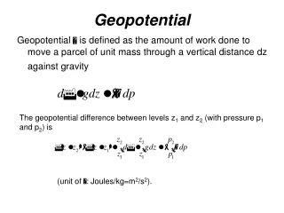
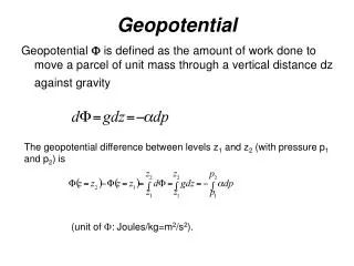
Geopotential. Geopotential is defined as the amount of work done to move a parcel of unit mass through a vertical distance dz against gravity. The geopotential difference between levels z 1 and z 2 (with pressure p 1 and p 2 ) is. (unit of : Joules/kg=m 2 /s 2 ). Dynamic height.

E N D
Geopotential Geopotential is defined as the amount of work done to move a parcel of unit mass through a vertical distance dz against gravity The geopotential difference between levels z1 and z2 (with pressure p1 and p2) is (unit of : Joules/kg=m2/s2).
Dynamic height , we have Given where is standard geopotential distance (function of p only) is geopotential anomaly. In general, is units of energy per unit mass (J/kg). However, it is call as “dynamic distance (D)” and sometime measured by the unit “dynamic meter” (1dyn m = 10 J/kg). Units: ~m3/kg, p~Pa, D~ dyn m Note: Though named as a distance, dynamic height (D) is a measure of energy per unit mass.
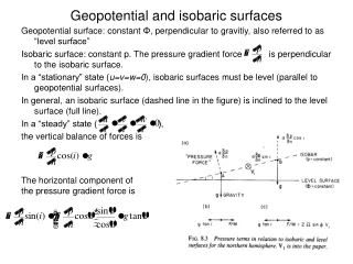
Geopotential and isobaric surfaces Geopotential surface: constant , perpendicular to gravity, also referred to as “level surface” Isobaric surface: constant p. The pressure gradient force is perpendicular to the isobaric surface. In a “stationary” state (u=v=w=0), isobaric surfaces must be level (parallel to geopotential surfaces). In general, an isobaric surface (dashed line in the figure) is inclined to the level surface (full line). In a “steady” state ( ), forces should be balanced. the vertical balance of forces is The horizontal component of the pressure gradient force is
Geostrophic relation The horizontal balance of force is where tan(i) is the slope of the isobaric surface. tan (i) ≈ 10-5 (1m/100km) if V1=1 m/s at 45oN (Gulf Stream). • In principle, V1 can be determined by tan(i). In practice, tan(i) is hard to measure because • p should be determined with the necessary accuracy • (2) the slope of sea surface (of magnitude <10-5) can not be directly measured (probably except for recent altimetry measurements from satellite.) (Sea surface is a isobaric surface but is not usually a level surface.)
Calculating geostrophic velocity using hydrographic data The difference between the slopes (i1 and i2) at two levels (z1 and z2) can be determined from vertical profiles of density observations. Level 1: Level 2: Difference: i.e., because A1C1=A2C2=L and B1C1-B2C2=B1B2-C1C2 because C1C2=A1A2 Note that z is negative below sea surface.
Since , and we have The geostrophic equation becomes
Current Direction • In the northern hemisphere, the current will be along the slope of a pressure surface in such a direction that the surface is higher on the right • In the northern hemisphere, the current flows relative to the water just below it with the “lighter water on its right” • Sverdrup et al. (The Oceans, 1946, p449) “In the northern hemisphere, the current at one depth relative to the current at a greater depth flows away from the reader if, on the average, the or t curves in a vertical section slope downward from left to right in the interval between two depths, and toward the reader if the curves slope downward from right to left”
Geostrophic Balance Magnitude of the current Horizontal pressure perpendicular to current direction
For two levels, Integrating along a line, L, linking stations A and B
“Thermal Wind” Equation Starting from geostrophic relation Differentiating with respect to z Using Boussinesq approximation (for the upper 1000 meters) Or Rule of thumb: light water on the right. .
Deriving Absolute Velocities • Assume that there is a level or depth of no motion (reference level) e.g., that V2=0 in deep water, and calculate V1 for various levels above this (the classical method) • When there are station available across the full width of a strait or ocean, calculate the velocities and then apply the equation of continuity to see the resulting flow is responsible, i.e., complies with all facts already known about the flow and also satisfies conservation of heat and salt • Use a “level of known motion”, e.g., if surface currents are known or if the currents have been measured at some depths. • Note that the bottom of the sea cannot be used as a level of no motion or known motion even though its velocity is zero.
Dynamic Topography at sea surface relative to 1000dbar (unit 0.1J/kgdynamic centimeter)
Relations between isobaric and level surfaces • A level of no motion is usually selected at about 1000 meter depth • In the Pacific, the uniformity of properties in the deep water suggests that assuming a level of no motion at 1000m or so is reasonable, with very slow motion below this • In the Atlantic, there is evidence of a level of no motion at 1000-2000 m (between the upper waters and the North Atlantic Deep Water) with significant currents above and below this depths • That the deep ocean current is small does not mean the deep ocean transport is small
Level of No Motion (LNM) Atlantic: A level of no motion at 1000-2000m above North Atlantic Deep Water Pacific: Deep water is uniform, current is weak below 1000m. “Slope current”: Relative geostrophic current is zero but absolute current is not. May occurs in deep ocean (barotropic). The situation is possible in deep ocean where T and S change is small Current increases into the deep ocean, unlikely in the real ocean
Neglecting small current in deep ocean affects total volume transport • Assume the ocean depth is 4000m, V=10 cm/s above 1000m based on zero current below gives a total volume transport for 4000m of 100m3/s • If the current is 2cm/s below 1000m, the estimate of V above 1000m has an error of 20% • The real total volume transport from surface to 4000m would be 180m3/s or 80% more than that assuming zero current below 1000m
Review Topics and Questions Properties of Sea Water • What unit of pressure is very similar to meter in depth in ocean? • What is salinity? Why can we use a single chemical constituent (which one?) to determine it? What other physical property of seawater is used to determine salinity? • What properties of seawater determine its density? What is an equation of state? • What happens to the temperature of a parcel of water (or any fluid or gas) when it is compressed adiabatically? What is potential temperature? Is it larger or smaller than the subsurface temperature? • What are the two effects of adiabatic compression on density? • What are t and ? How do they different from the in situ density? • Why do we use different reference pressure levels for potential density? • What factors determine the static stability?
Typical distribution of water properties • Major characteristics of the sea surface temperature (distributions of warm pool and cold tongue) and its seasonal cycle • Distribution of the surface salinity and its relation to the precipitation and evaporation • Typical vertical distribution of temperature. What is main thermocline? • What is seasonal thermocline? What are the major processes cause its formation?
Conservation laws • Mass conservation (continuity equation), volume conservation • Salt conservation (evaporation, river run-off, and precipitation) • Heat conservation (short and long-wave radiative fluxes, sensible and evaporative heat fluxes, basic factors controlling the fluxes, parameterizations) • Meridional heat and freshwater transports • Qualitative explanations of the major distributions of the surface heat flux components
Basic Dynamics • What are the differences between the centrifugal force and the Coriolis force? Why do we treat them differently in the primitive equation? • How to do a scale analysis for a fluid dynamics problem? • What is the hydrostatic balance? Why does it hold so well in the scales we are interested in? • What is the geostrophic balance? • What is the definition of dynamic height? • In geostrophic flow, what direction is the Coriolis force in relation to the pressure gradient force? What direction is it in relation to the velocity? • Why do we use a method to get current based on temperature and salinity instead of direct current measurements for most of the ocean? • How are temperature and salinity information used to calculate currents? What are the drawbacks to this method? • What is a "level of no motion"? Why do we need a "level of known or no motion" for the calculation of the geostrophic current? (What can we actually compute about the velocity structure given the density distribution and an assumption of geostrophy?)