The Phase Diagram module
The Phase Diagram module. Use the Phase Diagram module to generate various types of phase diagrams for systems containing stoichiometric phases as well as solution phases, and any number of system components. The Phase Diagram module accesses the compound and solution databases.

The Phase Diagram module
E N D
Presentation Transcript
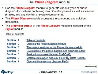
The Phase Diagram module • Use the Phase Diagram module to generate various types of phase diagrams for systems containing stoichiometric phases as well as solution phases, and any number of system components. • ThePhase Diagram module accesses the compound and solution databases. • The graphical output of the Phase Diagram module is handled by the Figure module. Table of contents Section 1Table of contents Section 2 Opening the Phase Diagram Module Section 3 The various windows of the Phase diagram module Section 4Calculation of the phase diagram and graphical output Section 5Predominance area diagram: Cu-SO2-O2 Section 6Metal-metal-oxygendiagram: Fe-Cr-O2 (Data Search) Section 7Classicalbinary phase diagram: Fe-Cr (continued) Phase Diagram 1.1
The Phase Diagram module Table of contents(continued) Section 8Metal-oxygendiagram: Fe-O2 Section 9Ternaryisoplethdiagram: Fe-C-W, 5 wt% W Section 10 Quaternarypredominance area diagram: Fe-Cr-S2-O2 Section 11Quaternaryisoplethdiagram: Fe-Cr-V-C, 1.5% Cr, 0.1% V Section 12Ternaryisothermaldiagram: CaO-Al2O3-SiO2 Section 13 Projections-Liquidus and First-Melting Section 14 Reciprocal Salt Polythermal Liquidus Projection Section 15 Paraequilibrium and Minimum Gibbs Energy Calculations Section 16Enthalpy-Composition (H-X) phase diagrams Appendix 1 Zero Phase Fraction (ZPF) Lines Appendix 2 Generalized rules for the N-Component System Appendix 3 Using the rules for classical cases: MgO-CaO, Fe-Cr-S2-O2 Appendix 4 Breaking the rules:H2O, Fe-Cr-C Phase Diagram 1.2
Initiating the Phase Diagram module Click on Phase Diagram in the main FactSage window. Phase Diagram 2
Components window – preparing a new Phase Diagram: CaO – SiO2 Calculation of the CaO-SiO2 binary phase diagram – T(C) vs. X(SiO2) 1°Click on the New button 2°Enter the first component, CaO and press the + button to add the second component SiO2. All examples shown here are stored in FactSage - click on: File > Directories… > Slide Show Examples … 3°PressNext >> to go to the Menu window The FACT Compound and solution databases are selected. Phase Diagram 3.1
Menu window – selection of the compound and solution species 1° Select the products to be included in the calculation: pure solid compound species and the liquid slag phase. 2° Right-click to display the extended menu on FACT-SLAG. 3° Select the option possible 2-phaseimmiscibility 4° Click in the Variables’ boxes to open the Variables window (or click on Variables in the menu bar). Phase Diagram 3.2
Compound species selection- FactSage 6.4 InFactSage 6.4 there is a new default exclusion of species from compound species selection When two or more databases are connected, the same species may appear in more than one database. In such cases, a species should generally only be selected from one database. Otherwise conflicts will probably occur. In order to assist users in deciding which species to exclude, the FactSage developers have assigned priorities. When you initially click on "pure solids", "pure liquids", or "gas" you may now see that several species marked with an "X" have not been selected. That is, they have been excluded by default because of probable conflicts between databases. The FactSage developers suggest that these species not be selected for this particular calculation. If you wish to select species marked with an "X" you must first click on 'permit selection of "X" species'. This will then override the default setting and permit you to select species as in FactSage 6.3. This will also activate the 'suppress duplicates' button and enable you to define a database priority list as in FactSage 6.3. IMPORTANT : For many calculations, it may frequently be advisable or necessary to de-select other species in addition to those marked with an "X." Phase Diagram 3.2.1
Compound species selection- FactSage 6.4 Fe + Cr + S2 + O2 using FactPS, FTmisc and FToxid databases. Right-click on ‘pure solids’ to open the Selection Window The species marked with an "X" have not been selected. The FactSage developers suggest that these species not be selected for this particular calculation. Phase Diagram 3.2.2
Compound species selection- FactSage 6.4 To override the default setting and select species marked with an "X“, click on 'permit selection of "X“ species'. You can then also set a database priority list and ‘Suppress Duplicates’. Phase Diagram 3.2.3
Variableswindow – defining the variables for the phase diagram Calculation of the CaO-SiO2 binary phase diagram – T(C) vs. X(SiO2) 2°PressNext >> to define the composition, temperature and pressure. 1° Select a X-Y (rectangular) graph and one composition variable: X(SiO2) 3° Set the Temperature as Y-axis and enter its limits. 4° Set the Pressure at 1 atm. 5° Set the composition [mole fraction X(SiO2)] as X-axis and enter its limits. 6° PressOK to return to the Menu window. Phase Diagram 3.3
Calculation of the phase diagram and graphical output 1°PressCalculate>> to calculate the phase diagram. Note the effect of the I option: the miscibility gap is calculated. 2° You can point and click to label the phase diagram. CaSiO3(s2) + Ca3Si2O7(s) See the Figure slide show for more features of the Figure module. Phase Diagram 4.1
A classical predominance area diagram In the following two slides is shown how the Phase Diagram module is employed in order to generate the same type of diagram that can also be produced with the Predom module. As an example the system isCu-SO2-O2. Note that SO2 and O2 are used as input in the Components window. Phase Diagram 5.0
Predominance area diagram: Cu-SO2-O2 1°Entry of the components(done in the Components window) • 2° Definition of the variables: • log10(PSO2), log10(PO2) • T = 1000K • P = 1 atm • 3°Selection of the products: • gas ideal • pure solids 4° Computation of the phase diagram Phase Diagram 5.1
Predominance area diagram: Cu-SO2-O2 ; Graphical Output Phase Diagram 5.2
A two metal oxygen system – Fe-Cr-O2 The following slides show how a phase diagram for an alloy system Fe-Cr-O2 with variable composition under a gas phase with variable oxygen potential (partial pressure) for constant temperature is prepared and generated. Note the use of the «metallic mole fraction» (Cr/(Cr+Fe)) on the x-axis and oxygen partial pressure log P(O2) on the y-axis. This example combines FACT (for the oxides) with SGTE (for the alloy solid solutions) databases. It shows ``Data Search`` and how to select the databases. Phase Diagram 6.0
Fe-Cr-O2: selection of databases 1°ClickData Search to open the Databases window. 2°Click on a box to include or exclude a database from the data search. Here the FACT and SGTE compound and solution databases have been selected. 3°PressNext >> to go to the Menu window Phase Diagram 6.1
Fe-Cr-O2: selection of variables and solution phases 1°Entry of the components(done in the Components window) • 2° Definition of the variables: • 1 chemical potential: P(O2) • 1 composition: XCr • T = 1573K • P = 1 atm • 3°Selection of the products: • gas ideal • pure solids • 5 solution phases 4° Computation of the phase diagram Phase Diagram 6.2
Fe-Cr-O2: graphical output Phase Diagram 6.3
A classical temperature vs composition diagram The following two slides show the preparation and generation of alabelled binary T vs X phase diagram. Note: The labels are entered into the diagram interactively. Click on the «A» button (stable phases label mode) and then move the cursor through the diagram. Where the left mouse button is clicked a label will be inserted into the diagram. The Fe-Cr system is used in this example. Phase Diagram 7.0
Fe-Cr binary phase diagram: input variables and solution species 1°Entry of the components(done in the Components window) • 2° Definition of the variables: • composition: 0 < WtCr< 1 • 500K < T < 2300K • P = 1 atm • 3°Selection of the products: • 4 solid solution phases • 1 liquid solution phase • Note the immiscibility for the BCC phase 4° Computation of the phase diagram Phase Diagram 7.1
Fe-Cr binary phase diagram: graphical output Phase Diagram 7.2
A two potential phase diagram In the following two slides the preparation and generation of a phase diagram with two potential axes is shown. The chosen axes are temperature and one chemical potential in a binary system. Note the difference in the diagram topology that results from the choice of RT ln P(O2) rather than log P(O2). The Fe-O2 system is used as the example. Phase Diagram 8.0
Fe-O2 system: input 1°Entry of the components(done in the Components window) • 2° Definition of the variables: • 1 chemical potential • 700K < T < 2000K • P = 1 atm • 3°Selection of the products: • pure solids • 4 solution phases 4° Computation of the phase diagram Phase Diagram 8.1
Fe-O2 system: graphical output Phase Diagram 8.2
A ternary isopleth diagram The following two slides show how a ternary isopleth diagram is prepared and generated. Temperature and one weight percent variable are used on the axes while the third compositional variable (here the wt% of the second metallic component) is kept constant. As an example the Fe-W-C system is used. Phase Diagram 9.0
Fe-C-W system at 5 wt% W: input 1°Entry of the components(done in the Components window) • 2° Definition of the variables: • 2 compositions (mass) • 900K < T < 1900K • P = 1 atm • 3°Selection of the products: • pure solids • 7 solution phases 4° Computation of the phase diagram Phase Diagram 9.1
Fe-C-W system at 5 wt% W: graphical output Phase Diagram 9.2
A quaternary predominance area diagram The following three slides show the preparation and calculation of a predominance area type phase diagram with two metal components and two gaseous components. The partial pressures, i.e. chemical potentials, of the gaseous components are used as axes variables. Note the use of the species names O2 and S2 in the Components window. These are used to retrieve the data for the correct gas species from the database. Temperature and total pressure are kept constant. Different from the Predom module the present diagram also shows the effect of solution phase formation (FCC, BCC, (Fe,Cr)S, Fe-spinel). As an example the Fe-Cr-S2-O2system is used. Phase Diagram 10.0
Predominance area diagram: Fe-Cr-S2-O2 System, solid solution input Note the chemical formula of the gas components. These are used because log pO2 and log pS2 are going to be axes variables. Phase Diagram 10.1
Fe-Cr-S2-O2System, variable and solid solution input 1°Entry of the components(done in the Components window) • 2° Definition of the variables: • 1 composition: XCr= 0.5 • 2 chemical potentials:P(O2) and P(S2) • T = 1273K • P = 1 atm • 3°Selection of the products: • solid (custom selection: an ideal solution) • 6 solution phases(including one with a possible miscibility gap) 4° Computation of the phase diagram Phase Diagram 10.2
Predominance area diagram: Fe-Cr-S2-O2 System, graphical output Phase Diagram 10.3
A quaternary isopleth diagram The following three slides show how the calculation of a quaternary isopleth diagram is prepared and executed. Furthermore, the use of the Point Calculation option is demonstrated. The resulting equilibrium table is shown and explained. As an example the Fe-Cr-V-C system is used. Phase Diagram 11.0
Fe-Cr-V-C system at 1.5 wt% Cr and 0.1 wt% V: input 1°Entry of the components(done in the Components window) • 2° Definition of the variables: • 3 compositions (1 axis) • 600°C < T < 1000°C • P = 1 atm • 3°Selection of the products: • 5 solid solutions(including 2 with possible miscibility gaps) 4° Computation of the phase diagram Phase Diagram 11.1
Fe-Cr-V-C system: graphical output With the phase equilibrium mode enabled, just click at any point on the diagram to calculate the equilibrium at that point. Phase Diagram 11.2
Fe-Cr-V-C system: phase equilibrium mode output Output can be obtained in FACT or ChemSage format. See Equilib Slide Show. Example is for FACT format. Proportions and compositions of the FCC phase (Remember the miscibility gap). NOTE: One of the FCC phases is metallic (FCC#1), the other is the MeC(1-x) carbide. Proportion and composition of the BCC phase. Phase Diagram 11.3
CaO-Al2O3-SiO2 ternary phase diagram: input 1°Entry of the components(done in the Components window) • 2° Definition of the variables: • 2 compositions (by default) • T = 1600°C • P = 1 atm • Gibbs triangle • 3°Selection of the products: • pure solids • Immiscible solution phase (FACT-SLAG) 4° Computation of the Gibbsternary phase diagram Phase Diagram 12.1
CaO-Al2O3-SiO2 ternary phase diagram: graphical output Phase Diagram 12.2
CaCl2-LiCl-KCl polythermal liquidus projection 1°Entry of the componentswith FTdemo database selected Parameterswindow – see next page • 2° Definition of the variables: • 2 compositions (by default) • T = projection • Step = 50 °C • P = 1 atm • 3°Selection of the products: • pure solids • solution phase (FTdemo-SALT) • option ‘P’ – Precipitation target 4° Computation of the univariant lines and liquidus isotherms Phase Diagram 13.1
CaCl2-LiCl-KCl polythermal liquidus projection : graphical output Click on Parameters intheMenuwindow Phase Diagram 13.2
Al2O3-CaO-SiO2 polythermal liquidus projection 1°Entry of the componentswith FToxid database selected • 2° Definition of the variables: • 2 compositions (by default) • T = projection • Max = 2600, Min = 1200, Step = 50 °C • P = 1 atm • 3°Selection of the products: • pure solids • solution phases • (FToxid-SLAGA) with • option ‘P’ – Precipitation target Phase Diagram 13.3
Al2O3-CaO-SiO2 polythermal liquidus projection : graphical output Phase Diagram 13.4
Zn-Mg-Al polythermal first melting (solidus) projection 1°Entry of the componentswith FTlite database selected • 2° Definition of the variables: • 2 compositions (by default) • T = projection • Step = 10 °C • P = 1 atm • 3°Selection of the products: • pure solids • solution phases • (FTlite-Liqu) with • option ‘F’ – Formation target • Note: The calculation of projections, particularly first melting sections, can be very time-consuming. Therefore, I and J options should not be used unless necessary. 4° Computation of the univariant lines and liquidus isotherms Phase Diagram 13.5
Zn-Mg-Al polythermal first melting (solidus) projection: graphical output Phase Diagram 13.6
Zn-Mg-Al isothermal section at 330 oC Note close similarity to the solidus projection of slide 13.6 Phase Diagram 13.7
Zn-Mg-Al liquidus projection Each ternary invariant (P, E) point on the liquidus projection corresponds to a tie-triangle on the solidus projection of slide 13.6 Phase Diagram 13.8
Zn-Mg-Al-Y First Melting (solidus) projection, mole fraction Yttrium = 0.05 Phase Diagram 13.9
When is a first melting projection not a solidus projection? - In systems with catatectics or retrograde solubility, a liquid phase can re-solidify upon heating. - In such systems, phase fields on a solidus projection can overlap. - However, “first melting temperature” projections never overlap. - If a system contains no catatectics or retrograde solubility (as is the case in the great majority of systems), the first melting temperature projection is identical to the solidus projection. - In systems with catactectics or retrograde solubility the first melting projection will exhibit discontinuities in temperature (and calculation times will usually be long). Phase Diagram 13.10.1
Ag-Bi, a system with retrograde solubility (SGTE database) Phase Diagram 13.10.2
Ag-Bi-Ge, First Melting Projection (SGTE database) Phase Diagram 13.10.3
Ce-Mn, a system with a catatectic (SGTE database) Phase Diagram 13.10.4
Ce-Ag, a system with a catatectic (SGTE database) Phase Diagram 13.10.5