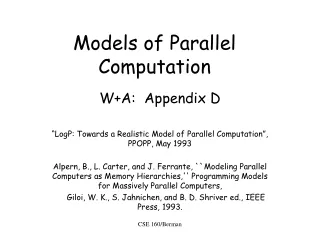
Models of Parallel Computation
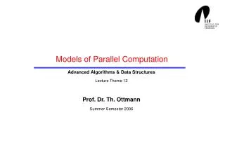
Models of Parallel Computation. Advanced Algorithms & Data Structures Lecture Theme 12 Prof. Dr. Th. Ottmann Summer Semester 2006. Overview. Models of parallel computation Characteristics of SIMD models Design issue for network SIMD models The mesh and the hypercube architectures

Models of Parallel Computation
E N D
Presentation Transcript
Models of Parallel Computation Advanced Algorithms & Data Structures Lecture Theme 12 Prof. Dr. Th. Ottmann Summer Semester 2006
Overview • Models of parallel computation • Characteristics of SIMD models • Design issue for network SIMD models • The mesh and the hypercube architectures • Classification of the PRAM model • Matrix multiplication on the EREW PRAM
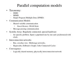
Models of parallel computation • Parallel computational models can be broadly classified into two categories, • Single Instruction Multiple Data (SIMD) • Multiple Instruction Multiple Data (MIMD)
Models of parallel computation • SIMD models are used for solving problems which have regular structures. We will mainly study SIMD models in this course. • MIMD models are more general and used for solving problems which lack regular structures.
SIMD models • An N- processor SIMD computer has the following characteristics : • Each processor can store both program and data in its local memory. • Each processor stores an identical copy of the same program in its local memory.
SIMD models • At each clock cycle, each processor executes the same instruction from this program. However, the data are different in different processors. • The processors communicate among themselves either through an interconnection network or through a shared memory.
Design issues for network SIMD models • A network SIMD model is a graph. The nodes of the graph are the processors and the edges are the links between the processors. • Since each processor solves only a small part of the overall problem, it is necessary that processors communicate with each other while solving the overall problem.
Design issues for network SIMD models • The main design issues for network SIMD models are communication diameter, bisection width, and scalability. • We will discuss two most popular network models, mesh and hypercube in this lecture.
Communication diameter • Communication diameter is the diameter of the graph that represents the network model. The diameter of a graph is the longest distance between a pair of nodes. • If the diameter for a model is d, the lower bound for any computation on that model is Ω(d).
Communication diameter • The data can be distributed in such a way that the two furthest nodes may need to communicate.
Communication diameter Communication between two furthest nodes takes Ω(d) time steps.
Bisection width • The bisection width of a network model is the number of links to be removed to decompose the graph into two equal parts. • If the bisection width is large, more information can be exchanged between the two halves of the graph and hence problems can be solved faster.
Bisection width Dividing the graph into two parts.
Scalability • A network model must be scalable so that more processors can be easily added when new resources are available. • The model should be regular so that each processor has a small number of links incident on it.
Scalability • If the number of links is large for each processor, it is difficult to add new processors as too many new links have to be added. • If we want to keep the diameter small, we need more links per processor. If we want our model to be scalable, we need less links per processor.
Diameter and Scalability • The best model in terms of diameter is the complete graph. The diameter is 1. However, if we need to add a new node to an n -processor machine, we need n - 1 new links.
Diameter and Scalability • The best model in terms of scalability is the linear array. We need to add only one link for a new processor. However, the diameter is n for a machine with n processors.
The mesh architecture • Each internal processor of a 2-dimensional mesh is connected to 4 neighbors. • When we combine two different meshes, only the processors on the boundary need extra links. Hence it is highly scalable.
The mesh architecture • Both the diameter and bisection width of an n-processor, 2-dimensional mesh is O(√n). • A 4 x 4 mesh
The hypercube architecture Hypercubes of 0, 1, 2 and 3 dimensions
The hypercube architecture • Each node of a d-dimensional hypercube is numbered using d bits. Hence, there are 2d processors in a d-dimensional hypercube. • Two nodes are connected by a direct link if their numbers differ only by one bit.
The hypercube architecture • The diameter of a d-dimensional hypercube is d as we need to flip at most d bits (traverse d links) to reach one processor from another. • The bisection width of a d-dimensional hypercube is 2d-1.
The hypercube architecture • The hypercube is a highly scalable architecture. Two d-dimensional hypercubes can be easily combined to form a d+1-dimensional hypercube. • The hypercube has several variants like butterfly, shuffle-exchange network and cube-connected cycles.
Adding n numbers on the mesh Adding n numbers in √nsteps
Adding n numbers on the hypercube Adding n numbers in log n steps