Models of Parallel Computation

1. Models of Parallel Computation W+A: Appendix D “LogP: Towards a Realistic Model of Parallel Computation”, PPOPP, May 1993 Alpern, B., L. Carter, and J. Ferrante, ``Modeling Parallel Computers as Memory Hierarchies,'' Programming Models for Massively Parallel Computers, Giloi, W. K., S. Jahnichen, and B. D. Shriver ed., IEEE Press, 1993. CSE 160/Berman

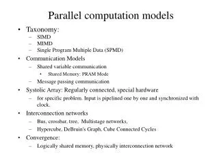
2. Computation Models • Model provides underlying abstraction useful for analysis of costs, design of algorithms • Serial computational models use RAM or TM as underlying models for algorithm design CSE 160/Berman

3. RAM [Random Access Machine] • unalterable program consisting of optionally labeled instructions. • memory is composed of a sequence of words, each capable of containing an arbitrary integer. • an accumulator, referenced implicitly by most instructions. • a read-only input tape • a write-only output tape CSE 160/Berman

4. RAM Assumptions • We assume • all instructions take the same time to execute • word-length unbounded • the RAM has arbitrary amounts of memory • arbitrary memory locations can be accessed in the same amount of time • RAM provides an ideal model of a serial computer for analyzing the efficiency of serial algorithms. CSE 160/Berman

5. PRAM [Parallel Random Access Machine] • PRAM provides an ideal model of a parallel computer for analyzing the efficiency of parallel algorithms. • PRAM composed of • P unmodifiable programs, each composed of optionally labeled instructions. • a single shared memory composed of a sequence of words, each capable of containing an arbitrary integer. • P accumulators, one associated with each program • a read-only input tape • a write-only output tape CSE 160/Berman

6. More PRAM • PRAM is a synchronous, MIMD, shared memory parallel computer. • Different protocols can be used for reading and writing shared memory. • EREW (exclusive read, exclusive write) • CREW (concurrent read, exclusive write) • CRCW (concurrent read, concurrent write) -- requires additional protocol for arbitrating write conflicts • PRAM can emulate a message-passing machine by logically dividing shared memory into private memories for the P processors. CSE 160/Berman

7. Broadcasting on a PRAM • “Broadcast” can be done on CREW PRAM in O(1): • Broadcaster sends value to shared memory • Processors read from shared memory CSE 160/Berman

8. LogP machine model • Model of distributed memory multicomputer • Developed by [Culler, Karp, Patterson, etc.] • Authors tried to model prevailing parallel architectures (circa 1993). • Machine model represents prevalent MPP organization: • machine constructed from at most a few thousand nodes, • each node contains a powerful processor • each node contains substantial memory • interconnection structure has limited bandwidth • interconnection structure has significant latency CSE 160/Berman

9. LogP parameters • L: upper bound on latency incurred by sending a message from a source to a destination • o: overhead, defined as the time the processor is engaged in sending or receiving a message, during which time it cannot do anything else • g: gap, defined as the minimum time between consecutive message transmissions or receptions • P: number of processor/memory modules CSE 160/Berman

10. LogP Assumptions • network has finite capacity. • at most ceiling(L/g) messages can be in transit from any one processor to any other atone time. • asynchronous communication. • latency and order of messages is unpredictable • all messages are small • context switching overhead is 0 (not modeled) • multithreading (virtual processes) may be employed but only up to a limit of L/g virtual processors CSE 160/Berman

11. LogP notes • All parameters measured in processor cycles • Local operations take one cycle • Messages are assumed to be small • LogP was particularly well-suited to modeling CM-5. Not clear if the same correlation is found with other machines. CSE 160/Berman

12. LogP Analysis of PRAM Broadcasting Algorithm • Algorithm: • Broadcaster sends value to shared memory (we’ll assume the value is in P0’s memory) • P Processors read from shared memory (other processors receive messages from P0) • Time for P0 to send P messages = o + g (P-1) • Maximum time for other processors to receive messages = o + (P-2)g + o + L + o CSE 160/Berman

13. g g g g L P0 P1 P2 P3 P4 P5 P6 P7 o o o o o o o o o o o o o o L L L L L L time Efficient Broadcasting in LogP Model Gap includes overhead time so overhead < gap CSE 160/Berman

14. 0 P0 g g g g L P0 P1 P2 P3 P4 P5 P6 P7 o o o o o o o o o o o o o o L P5 10 22 P1 L 14 18 L P3 P2 L L 20 24 24 L P7 P6 P4 time Mapping induced by LogP Broadcasting algorithm on 8 processors CSE 160/Berman

15. g g g g L P0 P1 P2 P3 P4 P5 P6 P7 o o o o o o o o o o o o o o L L L L L L time Analysis of LogP Broadcasting Algorithm to 7 Processors • Time to receive one message from P0 for first processor (P5) is L+2o • Time to receive message for last processor is max{3g+L+2o, 2g+L+2o, g+2L+4o, 4o+2L, g+4o+2L}=max{3g+L+2o, g+2L+4o} • Compare to LogP analysis of PRAM Broadcast which is o + (P-2)g + o + L + o = 5g + 3o + L CSE 160/Berman

16. 0 P0 P5 10 22 P1 14 18 P3 P2 20 24 24 P7 P6 P4 Scalable Performance • LogP Broadcast utilizes tree structure to optimize broadcast time • Tree depends on values of L,o,g,P • Strategy is much more scalable (and ultimately more efficient) than PRAM Broadcast CSE 160/Berman

17. Moral • Analysis can be no better than underlying model. The more accurate the model, the more accurate the analysis. • (This is why we use TM to determine undecidability but RAM to determine complexity.) CSE 160/Berman

18. Other Models used for Analysis • BSP (Bulk Synchronous Parallel) • Slight precursor and competitor to LogP • PMH (Parallel Memory Hierarchy) • Focuses on memory costs CSE 160/Berman

19. BSP[Bulk Synchronous Parallel] • BSP proposed by Valiant • BSP model consists of • P processors, each with local memory • Communication network for point-to-point message passing between processors • Mechanism for synchronizing all or some of the processors at defined intervals CSE 160/Berman

20. superstep synchronization superstep synchronization BSP Programs • BSP programs composed of supersteps • In each superstep, processors execute L computational steps using locally stored data, and send and receive messages • Processors synchronized at the end of the superstep (at which time all messages have been received) • BSP programs can be implemented through mechanisms like Oxford BSP library (C routines for implementing BSP programs) and BSP-L. CSE 160/Berman

21. superstep synchronization superstep synchronization BSP Parameters • P: number of processors (with memory) • L: synchronization periodicity • g: communication cost • s: processor speed (measured in number of time steps/second) • Processor sends at most h messages and receives at most h messages in a single superstep (communication called an h-relation) CSE 160/Berman

22. BSP Notes • Complete program = set of supersteps • Communication startup not modeled, g is for continuous traffic conditions • Message size is one data word • More than one process or thread can be executed by a processor. • Generally assumed that computation and communication are not overlapped • Time for a superstep = max number of local operations performed by any processor + g(max number of messages sent or received by a processor) + L CSE 160/Berman

23. BSP Analysis of PRAM Broadcast • Algorithm: • Broadcaster sends value to shared memory (we’ll assume the value is in P0’s memory) • P Processors read from shared memory (other processors receive messages from P0) • In BSP model, processors only allowed to send or receive at most h messages in a single superstep. Broadcast for more than h processors would require a tree structure • If there were more than Lh processors, then a tree broadcast would require more than one superstep. • How much time does it take for a P processor broadcast? CSE 160/Berman

24. h-ary tree … … … BSP Analysis of PRAM Broadcast • How much time does it take for a P processor broadcast? CSE 160/Berman

25. PMH [Parallel Memory Hierarchy] Model • PMH seeks to represent memory. Goal is to model algorithms so that good decisions can be made about where to allocate data during execution. • Model represents costs of interprocessor communication and memory hierarchy traffic (e.g. between main memory and disk, between registers and cache). • Proposed by Carter, Ferrante, Alpern CSE 160/Berman

26. PMH Model • Computer is modeled as a tree of memory modules with the processors at the leaves. • All data movement takes the form of block transfers between children and their parents. • PMH is composed of a tree of modules • all modules hold data • leaf modules also perform computation • data in a module is partitioned into blocks • Each module has 4 parameters for each module CSE 160/Berman

27. Shareddisk system network network Caches Disks Caches Disks Disks Disks Disks Disks Disks Mainmemories Mainmemories ALU/registers ALU/registers Un-parameterized PMH Models for a Cluster of Workstations Bandwidth from processor to disk> bandwidth from processor to network Bandwidth between 2 processors> bandwidth to disk CSE 160/Berman

28. PMH Module Parameters • Blocksizes_m tells how many bytes there are per block of m • Blockcountn_m tells how many blocks fit in m • Childcountc_m tells how many children m has • Transfer timet_m tells how many cycles it takes to transfer a block between m and its parent • Size of "node" and length of "edge" in PMH graph should correspond to blocksize, blockcount and transfer time • Generally all modules at a given level of the tree will have the same parameters CSE 160/Berman

29. Summary • Goal of parallel computation models is to provide a realistic representation of the costs of programming. • Model provides algorithm designers and programmers a measure of algorithm complexity which helps them decide what is “good” (i.e. performance-efficient) • Next up: Mapping and Scheduling CSE 160/Berman