Genetic Design for Composite Interval Mapping: QTL Analysis and Simulation Framework
This program is designed for researchers conducting Composite Interval Mapping (CIM) in genetic studies. The tool allows users to input cumulative marker distances and trait data for simulating QTL searching. It provides analysis options for handling controlled background markers and implements permutation tests to establish significance thresholds. The framework supports backcross and F2 populations, enabling users to estimate genetic effects accurately while assessing the presence of QTLs at specified locations. This program promotes robust genetic analysis and facilitates advanced simulations in plant and animal breeding research.

Genetic Design for Composite Interval Mapping: QTL Analysis and Simulation Framework
E N D
Presentation Transcript
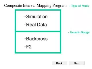
CompositeInterval Mapping Program - Type of Study - Genetic Design
CompositeInterval Mapping Program - Data and Options Cumulative Marker Distance (cM) Map Function QTL Searching Step cM Parameters Here for Simulation Study Only
CompositeInterval Mapping Program - Data Put Markers and Trait Data into box below OR
CompositeInterval Mapping Program - Analyze Data For CIM, Controlled Background Markers by Within cM Or Markers
CompositeInterval Mapping Program - Profile
CompositeInterval Mapping Program - Permutation Test #Tests Cut Off Point at Level Is Based on Tests.
r=a+b-2ab M a Q b N F2 Population – Three Point
Composite model for interval mapping and regression analysis zi: QTL genotype xik: marker genotype yi = + a* zi + km-2bkxik + ei Expected means: Qq: + a* + kbkxik = a* + XiB qq: + kbkxik = XiB Xi = (1, xi1, xi2, …, xi(m-2))1x(m-1) B = (, b1, b2, …, bm-2)T M1 x1 M1m1 1 +b1 m1m1 0
zi – conditional probability of Qq given markers of individual i and QTL position xik – coding for ‘effect’ of k-th marker of i Backcross: xik =1 if k-th marker of i is Mm =0 or –1 if k-th marker of i is mm km-2 – summation over all markers except two markers of current interval We want estimate a* and test if abs(a*) is big enough to claim that there is a QTL at the given location in an interval. The estimate B is not very important
Likelihood based CIM L(y,M|) = i=1n[1|if1(yi) + 0|if0(yi)] log L(y,M|) = i=1n log[1|if1(yi) + 0|if0(yi)] f1(yi) = 1/[(2)½]exp[-½(y-1)2], 1= a*+XiB f0(yi) = 1/[(2)½]exp[-½(y-0)2], 0= XiB Define 1|i= 1|if1(yi)/[1|if1(yi) + 0|if0(yi)] (1) 0|i= 0|if1(yi)/[1|if1(yi) + 0|if0(yi)] (2)
a* = i=1n1|i(yi-a*-XiB)/ i=1n1|i (3) = 1 (Y-XB)´/c B = (X´X)-1X´(Y-1a*) (4) 2 = 1/n (Y-XB)´(Y-XB) – a*2 c (5) • = (i=1n21|i +i=1n30|i)/(n2+n3) (6) Y = {yi}nx1, = {1|i}nx1, c = i=1n1|i
Hypothesis test H0: a*=0 vs H1: a*0 L0 = i=1nf(yi) B = (X´X)-1X´Y, 2=1/n(Y-XB)´(Y-XB) L1= i=1n[1|if1(yi) + 0|if0(yi)] LR = -2(lnL0 – lnL1) LOD = -(logL0 – logL1)
Likelihood based CIM for BC and F2 L(y,M|) = i=1n k=1g [k|ifk(yi)] log L(y,M|) = i=1n log[k=1gk|ifk(yi)] g=2 for BC, 3 for F2 fk(yi) = 1/[(2)½]exp[-½(y-k)2], k= gk+XiB k=1,…,g
Define k|i= k|if1(yi)/[k=1gk|if1(yi)] (1) B = k=1gk(X´X)-1X´(Y- gk) (2) gk = i=1nk|i(yi-XiB)/ i=1nk|i (3) 2 = 1/n i=1n k=1gk|i(yi-XiB - gk )2 (4) Y = {yi}nx1, k= {k|i}nx1