CacheMiner : Run-Time Cache Locality Exploitation on SMPs
120 likes | 155 Views
Learn how to exploit on-chip/cache and off-chip/cache for improved data access performance in nested-loop structures. Includes compiler hints, task grouping, partitioning, and scheduling strategies.

CacheMiner : Run-Time Cache Locality Exploitation on SMPs
E N D
Presentation Transcript
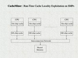
CacheMiner : Run-Time Cache Locality Exploitation on SMPs CPU CPU CPU On-chip cache On-chip cache On-chip cache Off-chip cache Off-chip cache Off-chip cache Interconnection Network Shared Memory
Example Program transformations for cache locality : Tiling for i = 1 to n for j = 1 to n for k = 1, n A[i,j ] = A[i,j] + B[i,k] * C[k,j] For a matrix multiplication of 1000 x 1000 … = X Data accessed 1000 1000 1000 1002000 = X 1000 1000 32 32 32 65024 = X 1000
But it’s hard for the compiler to analyse indirect accesses.. void myfunc( int source_arr[] , int key_arr[] , int result_arr[], int n) { for(I=0;I< n ;I++) { result_arr[I] += source_arr[key_arr[ I]] ; // Indirection ! } } • The data access pattern of the function depends on the • contents of key_arr[] . • So the data access pattern cannot be determined at compile • time, but only at run-time. • Cacheminer is especially useful for such scenarios.
Targetted Model For ( i1 = lower_1 ; i1 < upper_1 ; i1 ++) For ( i2 = lower_2 ; i2 < upper_2 ; i2 ++) For ( i3 = lower_3 ; i3 < upper_3 ; i3 ++) k nested loops For ( ik = lower_k ; ik < upper_k ; ik ++) { Task B = block of statements; } Let B ( t1, t2…tk) : task B where t1 , t2..tk represent particular values of variables i1 , i2 ..ik respectively The tasks need to be data independent of each other i.e : Out (B1) Out (B2) = { empty set } Out (B1) In (B2) = { empty set } In (B1) Out (B2) = { empty set }
System Overview program • C program • Add calls to library functions which provide hints • to the run-time system • Use Hints to estimate the pattern of accesses. • Group together tasks which access closely placed • data into bins . • Partition total bins among P processors to maximize • data locality and also loadsharing. • Schedule Tasks on the processor. Ensure overall • load-balancing Hint Addition Library Compiler Access Pattern Estimation 1 2 Task Grouping Task Partitioning 3 Task Scheduling 4
Step 1 : Estimating Memory Accesses • Assumption : Task B accesses only chunks of elements in multiple arrays • 4 Hints provided to the module : • a. Number of Arrays accessed : n (Compile Time) • b. Size in bytes of each array : Vector (s1,s2…sn) (Compile Time) • c. Number of processors : p (Compile Time). • d. Access footprintB(a1,a2,….an) : starting access address • for n arrays for the Task B. (Run Time). • Each Task can then be a point B(a1,a2,a3..an) in n -dimensional space.
Example : int P [ 100 ] and int Q[ 200]. Memory Layout of P : size = 100 * sizeof(int) = 400 : starting address : &P[0] = 1000 Memory Layout of Q : size = 200 * sizeof(int) = 800 : starting address : &Q[0] = 100. B1 ( 1000, 900) 900 Access dimension in Q --> 100 B2 ( 1000, 100) 1000 1400 Access dimension in P --> Each Task B(x ,y) is a point in the 2-dimensional grid x : starting access address of array1 (P) for Task y : starting access address of array2 (Q) for Task
Step 2 : Grouping Tasks By Locality A. Shift to Origin. B1 ( 1000, 900) 900 800 Access dimension in Q --> 100 B2 ( 1000, 100) 0 400 1000 1400 Access dimension in P --> B. Shrink the Dimensions by (C/n) : 8 Bins In example : n = 2, cache size = 200 So shrink dimension by 200/2 = 100 0 4
Step 3 : Partitioning Bins among ‘P’ Processors • Need to form ‘P’ groups of bins such that the sharing between them is • minimized. • Problem is NP-complete, so use a heuristic method to divide up the bin • space. • i. Form prime factors of ‘P’ and divide each dimension of bin-space • into Rj chunks , for each Prime factor Rj. Example : Suppose we have 6 processors : 6 = 2 x 3 So ‘x’ dimension divided into 2 parts. ‘y’ dimension divided into 3 parts. Thus, a total of 2 x 3 = 6 distinct regions ! (all bins in 1 region are processed by one processor). Distinct regions 8 0 4
Step 4 : Adaptive Scheduling of Task Groups Bin Bin Bin Bin Bin Bin Processor Task List Take ‘K’ bins at a time Local Scheduling : Each processor processes bins from its own Task-list. Global Scheduling : When a processor finishes its task list, it starts processing the task list of the most heavily loaded processor. Adaptive Control : Processor takes ‘K’ bins at a time to process. K changes depending on no. of remaining bins max ( p /2 , Ki - 1) if few bins remain in tasklist (light load) min ( 2p , Ki + 1) if lots of bins remain in tasklist (heavy load) Ki =
With Cacheminer Results Manually optimized Static Access Pattern Static Access Pattern Dynamic Access Pattern
Summary • Framework to exploit Run-Time Cache Locality on SMPs • Targetted at nested-loop structures accessing number of arrays. • Especially useful for indirect accesses where data access pattern • cannot be determined till run-time. • Overall phases : Hint Addition program Access Pattern Estimation Task Grouping Compiler Task Partitioning Library Task Scheduling