Download
1 / 44
440 likes | 575 Views
Automated Ranking Of Database Query Results. Sanjay Agarwal - Microsoft Research Surajit Chaudhuri - Microsoft Research Gautam Das - Microsoft Research Aristides Gionis - Computer Science Dept

E N D
Automated Ranking Of Database Query Results Sanjay Agarwal - Microsoft Research Surajit Chaudhuri - Microsoft Research Gautam Das - Microsoft Research Aristides Gionis - Computer Science Dept Stanford University Presented at the first Conference on Innovative Data Systems Research (CIDR) in the year 2003 Ramya Somuri Nov ‘10 2009
Outline • Introduction • Problem Formulation • Similarity Functions • Implementation • Experiments • Conclusion
Boolean Semantics of SQL: Success and Barrier? Example: Select * From Realtor R Where 400K<Price<600K AND #Bedrooms= 4 Problems: • Query Semantics: • True/False { BOOLEAN MODEL} • Query Results Representation: • Empty Answers • Many Answers A Ranked List Similarity, Relevance, Preference What do we want? What do we want?
Empty answers problem • In this case it would be desirable to return a ranked list of ‘approximately’ matching tuples without burdening the user to specify any additional conditions. • In other words, an automated approach for ranking and returning approximately matching tuples.
What is Ranking? • As the name suggests ‘Ranking’ is the process of ordering a set of values (or data items) based on some parameter that is of high relevance to the user of ranking process. • Ranking and returning the most relevant results of user’s query is a popular paradigm in information retrieval.
What is Automated Ranking? • Automated ranking of query results is the process of taking a user query and mapping it to a Top-K query with a ranking function that depends on conditions specified in the user query.
Focus of Paper Develop a method for automatically ranking database records by relevance to a given query Derive a Similarity Function Apply Similarity Function between Query & Records in database Rank the Result-Set and return Top-K records
Automated Ranking functions for the ‘Empty Answers Problem’ • IDF Similarity - Mimics the TF-IDF concept for Heterogeneous data. • QF Similarity - Utilizes workload information. • QFIDF Similarity - Combination of QF and IDF.
Attributes Categorical Attribute Numerical Attribute T u p l es Vk
Notations: • R - Relation • {Al,…,Am} - Set of Attributes • Vk – Set of valid attribute values for an attribute Ak • {tl,……,tm} - Tuples/records • A tuple t is expressed as t = <tl,……tm> for a tuple with values tk ε Vk for each k • Q - <Tl,…..Tm>
Notations: • Where clause of Query Q is of the form “WHERE Cl AND …….AND Ck” Each Ci is of the form Ai IN {valuel,………..,valuek} / Ai IN [lb,ub] • Similarity coefficient Sk(u,v) can be defined as “similarity” for the attribute values [u,v] • Sk(u,v) =1 if u=v =0 if u,v are dissimilar • Wk – “importance” of attribute/Attribute weight 0<wk<1; Σwk=1
w IDF Similarity • Database(only categorical attribute) • T=<t1,……tm> • Q=<q1,…...qm> Condition is “WHERE is A1=q1” • IDFk(t)=log(n/Fk(t)) • n-number of tuples in database • Fk(t) -Frequency of tuples in database where Ak=t • Similarity between T and Q is • Sum of corresponding similarity coefficients over all attributes • Dot product is un-normalized • TF is irrelevant • Similarity function known as IDF similarity <attribute,value> d tuple IR technique Q = set of key words IDF(w) = log(N/F(w)) N - No of documents F(w) - No of occurrences of documents in which w appears TF(w,d)=Frequency of occurrence of w in d Cosine similarity between query and document is normalized dot product of the two corresponding vector Similarity function known as cosine similarity with TF-IDF weightings
IDF Similarity Example • Select model from automobile_database Where TYPE=“convertible” and MFR=“Nissan”; • System generates tuples in the following order • Nissan Convertibles • Convertibles by other manufacturer • Other cars/types by Nissan • “Convertible” is rare and has higher IDF than “Nissan” which is a common car manufacturer
Can we use IDF Similarity SIM(T,Q) to Numerical Atributes? • No • Example Select * From automobile_database Where price=3000 • Sk(u,v) = 1 if (u=v) otherwise 0 is a bad definition since two numerical values might be close but not equal.
Some suggested Sk(u,v) for numerical data • Sk(u,v) = 1-d/ | uk-lk | where d=|v-u| is the distance between the value & [lk,uk] is the domain of Ak • Example: Select * from Realtor R where #rooms=4
Generalizations of IDF similarity • For numeric data • Inappropriate to use previous similarity coefficients/functions. • frequency of numeric value depends on nearby values. • Discretizing numeric to categorical attribute is problematic. • Solution: • {t1,t2…..tn} be the values of attribute A. For every value t, • Similarity function is • sum of ”contributions” of t from every other point it contributions modeled as Gaussian distribution
Shortcomings with IDF Similarity • Problem: In a realtor database, more homes are built in recent years such as 2007 and 2008 as compared to 1980 and1981. Thus recent years have small IDF.Yet newer homes have higher demand. • Solution: QF Similarity.
QF Similarity : leveraging workloads • Importance of attribute values is directly related to the frequency of their occurrence in workload. • In the previous example, it is reasonable to assume that more queries are requesting for newer homes than for older homes. Thus the frequency of the year 2008 appearing in the workload will be more than that of year 1981.
QF Similarity : leveraging workloads • Query frequency QF(q) = RQF(q)/ RQFMax RQF(q) - raw frequency of occurrence of value q of attribute A in query strings of workload RQFMax - raw frequency of most frequently occurring value in workload • S(t,q)= QF(q), if q=t 0 , otherwise
QF Similarity example Consider a workload W = { Q1,Q2,Q3,Q4} Q1- Select * from Realtor R where year=“2009” Q2- Select * from Realtor R Where year=“2009” Q3- Select * from Realtor R Where year=“2008” Q4- Select * from Realtor R Where year=“2007” Attribute Year= { 1981,……., 2009} QF (2008) = RQF(2008)/RQFMax = 1/2 . If a query requests for an attribute value not in the workload, then QF=0. Ex- QF(1981)=0
QF Similarity : Different Attributes • Problem/Example: SMFR(Toyota,Honda) =0 SMODEL (Camry, Accord) =0 • Solution: Similarity Coefficients that are non-zero even when the pair of categorical attributes is different Eg:SMFR(Toyota,Honda) =0.9
QF Similarity : Different Attributes • Similarity between pairs of different categorical attribute values can also be derived from workload • The similarity coefficient between tuple and query in this case is defined by jaccard coefficient scaled by QF factor as shown below. S(t,q)=J(W(t),W(q))QF(q)
Analyzing workloads • Analyzing IN clauses of queries: If certain pair of values often occur together in the workload ,they are similar .e.g. queries with C as “MFR IN {TOYOTA,HONDA,NISSAN}” • Several recent queries in workload by a specific user repeatedly requesting for TOYOTA and HONDA. • Numerical values that occur in the workload can also benefit from query frequency analysis.
QFIDF Similarity Why QFIDF? • QF is purely workload-based. • Doesn't use data at all. • Fails in case of insufficient & unreliable workloads. What is QFIDF? • QFIDF is a hybrid ranking function obtained by combing IDF, QF weights by multiplying them • For QFIDF Similarity • S(t,q)=QF(q) *IDF(q) ,when t=q 0, otherwise where QF(q)=(RQF(q)+1)/(RQFMax+1). • Thus we get small non zero QF even if value is never referenced in workload model.
Breaking ties…. • In case of many answers problem, the recently discussed ranking functions might fail to perform. • This is because many tuples may tie for the same similarity score. Such a scenario could arise for empty answer problem also. • To break this tie, requires looking beyond the attributes specified in the query, i.e., missing attributes.
Breaking ties using QF • Solution: Determine the weights of missing attribute values that reflect their “global importance” for ranking purposes by using workload information. • Extend QF similarity ,use quantity Σlog(QFk(tk)) to break ties. Consider a query requesting for 4 bedroom houses . • Result set= many # of homes • Examine the other attributes other than # of bed rooms(missing attributes). Ex- Location - Dallas is more important than Arlington . • Rank the 4 bed room homes in Dallas higher than that of Arlington
Problems with Breaking ties using IDF • Rank the tuples with large IDF for missing attributes higher • Arlington homes are given more preference than Dallas homes since Arlington has a higher IDF, but this scenario is not true in real practice. • Rank the tuples with small IDF for missing attributes higher Consider homes with decks , but since we are considering smaller IDF preference will be given to homes without decks since they have a smaller IDF which is not true in real practice.
Implementation • Pre-processing component • Query–processing component
Pre-processing component • Compute and store a representation of similarity function in auxiliary database tables. • For categorical data: ComputeIDF(t) (resp QF(t)) ,to compute frequency of occurrences of values in database and store the results in auxiliary database tables. • For numeric data: An approximate representation of smooth function IDF() (resp(QF()) is stored, so that function value of q is retrieved at runtime.
Query processing component • Main task: Given a query Q and an integer K, retrieve Top-K tuples from the database using one of the ranking functions. • Ranking function is extracted in pre-processing phase. • SQL-DBMS functionality used for solving top-K problem. • Handling simpler query processing problem • Input: table R with M categorical columns, Key column TID, C is conjunction of form Ak=qk..... and integer K. • Output: top-K tuples of R similar to Q. • Similarity function: Overlap Similarity.
Implementation of Top-K operator • Traditional approach ? • Indexed based approach • overlap similarity function satisfies the following monotonic property. • If T and U are two tuples such that for all K, Sk(tk,qk)< Sk(uk,qk) then SIM(T,Q) < SIM(U,Q) • To adapt TA implement Sorted and Random access methods. • Performs sorted access for each attribute, retrieve complete tuples with corresponding TID by random access and maintains buffer of Top-K tuples seen so far.
d: 0.9 a: 0.85 b: 0.7 . . . . c: 0.2 Threshold Algorithm (TA) • Read all grades of an object once seen from a sorted access • No need to wait until the lists give k common objects • Do sorted access (and corresponding random accesses) until you have seen the top k answers. • How do we know that grades of seen objects are higher • than the grades of unseen objects ? • Predict maximum possible grade unseen objects: L2 L1 a: 0.9 Seen b: 0.8 c: 0.72 T = min(0.72, 0.7) = 0.7 f: 0.6 . . . . f: 0.65 Possibly unseen Threshold value d: 0.6
ID L2 L1 (d, 0.9) (a, 0.9) (b, 0.8) (a, 0.85) (c, 0.72) (b, 0.7) A1 Min(A1,A2) A2 . . . . . . . . (d, 0.6) (c, 0.2) Example – Threshold Algorithm Step 1: - parallel sorted access to each list For each object seen: - get all grades by random access - determine Min(A1,A2) - amongst 2 highest seen ? keep in buffer a 0.9 0.85 0.85 0.6 0.9 0.6 d
ID L2 L1 a: 0.9 d: 0.9 a: 0.85 b: 0.8 a 0.9 b: 0.7 c: 0.72 0.9 d A2 Min(A1,A2) A1 . . . . . . . . d: 0.6 c: 0.2 Example – Threshold Algorithm Step 2: - Determine threshold value based on objects currently seen under sorted access. T = min(L1, L2) - 2 objects with overall grade ≥ threshold value ? stop else go to next entry position in sorted list and repeat step 1 0.85 0.85 0.6 0.6 T = min(0.9, 0.9) = 0.9
ID L2 L1 (a, 0.9) (d, 0.9) (b, 0.8) (a, 0.85) (c, 0.72) (b, 0.7) A1 A2 Min(A1,A2) . . . . . . . . (d, 0.6) (c, 0.2) Example – Threshold Algorithm Step 1 (Again): - parallel sorted access to each list For each object seen: - get all grades by random access - determine Min(A1,A2) - amongst 2 highest seen ? keep in buffer a 0.9 0.85 0.85 d 0.6 0.9 0.6 b 0.8 0.7 0.7
ID L2 L1 a: 0.9 d: 0.9 a: 0.85 b: 0.8 a 0.9 b: 0.7 c: 0.72 0.7 b A2 Min(A1,A2) A1 . . . . . . . . d: 0.6 c: 0.2 Example – Threshold Algorithm Step 2 (Again): - Determine threshold value based on objects currently seen. T = min(L1, L2) - 2 objects with overall grade ≥ threshold value ? stop else go to next entry position in sorted list and repeat step 1 0.85 0.85 0.7 0.8 T = min(0.8, 0.85) = 0.8
ID L2 L1 a: 0.9 d: 0.9 a: 0.85 b: 0.8 a 0.9 b: 0.7 c: 0.72 0.7 b A2 Min(A1,A2) A1 . . . . . . . . d: 0.6 c: 0.2 Example – Threshold Algorithm Situation at stopping condition 0.85 0.85 0.7 0.8 T = min(0.72, 0.7) = 0.7
Indexed-based TA(ITA) Sorted access Random access
Indexed-based TA(ITA) Stopping Condition • Hypothetical tuple – current value a1,…, ap for A1,… Ap, corresponding to index seeks on L1,…, Lp and qp+1,….. qm for remaining columns from the query directly. • Termination – Similarity of hypothetical tuple to the query< tuple in Top-k buffer with least similarity.
Conclusion • Automated Ranking Infrastructure for SQL databases. • Extended TF-IDF based techniques from Information retrieval to numeric and mixed data. • Implementation of Ranking function that exploited indexed access (Fagin’s TA)