Download
1 / 65
650 likes | 785 Views
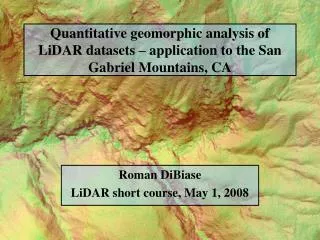
Quantitative geomorphic analysis of LiDAR datasets – application to the San Gabriel Mountains, CA. Roman DiBiase LiDAR short course, May 1, 2008. Quantitative analysis of topography using LiDAR.

E N D
Quantitative geomorphic analysis of LiDAR datasets – application to the San Gabriel Mountains, CA Roman DiBiase LiDAR short course, May 1, 2008
Quantitative analysis of topography using LiDAR • Airborne laser swath mapping (ALSM) consistently provides data good enough to produce 1m digital elevation models (DEMs) • Ground-based systems can be used for finer scale analysis of millimeter to centimeter scale features • These datasets are more than just pretty pictures; many important research questions have become testable as a result of this technology
There are many cases where detailed terrain modeling is needed • Geomorphic mapping • fault scarps, landslides, stream terraces • Geomorphic process studies • soil production rates, soil transport model testing • knickpoint form, channel geometry/morphology • Landscape monitoring • repeat scans using ground-based LiDAR
Alternatives to LiDAR • Total station surveys • Time consuming!! • Photogrammetry • Tree cover • Expensive
SAF = San Andreas Fault SMF = Sierra Madre Fault CF = Cucamonga Fault SGF = San Gabriel Fault = igneous/metamorphic rocks Field Area: San Gabriel Mountains, CA 30 km N modified from Blythe et al., 2000
Local relief (1km radius) West-to-east gradient in uplift rate from low to high can be inferred from topography, quaternary slip rates, and low-temperature thermochronometry work
How do we obtain appropriate erosion rates? • Thermochron cooling ages range from 3-60 Ma • Even using geologic constraints, the inferred erosion rates are averaged over millions of years • We need more geomorphically appropriate rates, on the order of landform development…
10Be is produced in quartz grains through the interaction of cosmic rays with oxygen nuclei
Quartz grains accumulate 10Be during their path from bedrock to stream sand Quartz grains accumulate 10Be proportional to the time they spend within the top meter or so of Earth’s surface.
Alluvial sand samples average exposure ages of millions of grains By analyzing a bag of sand (~1 kg) in bulk we are in effect averaging over the entire area draining to the sample
Catchment-averaged sample location map So far, erosion rates range from ~10 – 1000 m/My
OK, now that we have erosion rates… • There are a few main questions we can tackle now • How does hillslope form vary with erosion rate? • What is the erosion rate threshold for hillslope sensitivity? • How does channel steepness vary with erosion rate? • Do channels have a similar threshold? • Does channel width vary with erosion rate? • How are conditions different across transition zones (knickpoints)? • How replicable are basin cosmo rates in bedrock landscapes?
Which processes are acting to lower the landscape? • Hillslope processes • Channel incision • Debris flow scour • Bedrock landsliding
Which processes are acting to lower the landscape? • Hillslope processes • Channel incision • Debris flow scour • Bedrock landsliding Most understood!
Channel long profile analysis • Well-adjusted channel profiles tend to follow a power-law relationship between slope and drainage area S = ks A- • ks = channel steepness index: varies with uplift, climate, lithology • = concavity index: independent of uplift rate elevation log S distance log A
Slope-area plots extracted from 10m DEMs Cattle Creek
Slope-area plots extracted from 10m DEMs Fluvial regime S=ksnA-0.45 Cattle Creek Debris flow regime?
Slope-area plots extracted from 10m DEMs Channel steepness index, ksn Cattle Creek
Spatial variations in erosion rates red = high uplift zone blue = low uplift zone
Temporal variations in erosion rates Bear Creek
Temporal variations in erosion rates Bear Creek knickpoint knickpoint
Temporal variations in erosion rates Bear Creek knickpoint ksn = 192 ksn = 86 knickpoint
Map of channel steepness index variation Green= low channel steepness Red = high channel steepness
Tutorial • Channel network extraction • How do we define a channel? • Scale issues • What problems do we run into when using high-resolution elevation data? • Resampling high-resolution data • Techniques to probe datasets • Extracting elevation profiles, slope profiles
Pretty darn good, though there are some funny offsets ~12m offset ~25m offset
Stream extracted from 2m LiDAR DEM follows a tortuous path around large boulders, etc. Channel is much wider than 1 pixel! At high flow,channel is ~15-20m wide 100m
LiDAR contributions to understanding channel processes • Flow paths are often wrong with high-res data, meaning drainage areas are troublesome to determine • Local channel slope is underestimated in some cases due to critical jump in scale to less than channel width • Despite this, lidar data contain valuable information concerning knickpoint form, width variation, and potentially bed roughness
What can hillslopes tell us about erosion rates? Hypothesis: With increasing erosion rates, slopes steepen, soil thickness decreases, but once maximum soil production rate is exceeded, threshold, landsliding slopes dominate