Download
1 / 45
460 likes | 617 Views
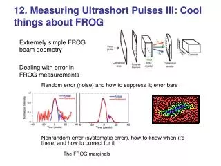
12. Measuring Ultrashort Pulses III: Cool things about FROG. Extremely simple FROG beam geometry . Dealing with error in FROG measurements Random error (noise) and how to suppress it; error bars Nonrandom error (systematic error), how to know when it’s there, and how to correct for it

E N D
12. Measuring Ultrashort Pulses III: Cool things about FROG Extremely simple FROG beam geometry Dealing with error in FROG measurements Random error (noise) and how to suppress it; error bars Nonrandom error (systematic error), how to know when it’s there, and how to correct for it The FROG marginals
Pulse to be measured SHG crystal SHG crystal Camera Can we simplify FROG? FROG has 3 sensitive alignment degrees of freedom (q, f of a mirror and also delay). The thin crystal is also a pain. Pulse to be measured Camera Spec- trom- eter Variable delay 2 alignment q parameters q (q, f) q Crystal must be very thin, which hurts sensitivity. 1 alignment q parameter q (delay) q Remarkably, we can design a FROG without these components!
GRating-Eliminated No-nonsense Observationof Ultrafast Incident Laser Light E-fields(GRENOUILLE) FROG 2 key innovations: A single optic that replaces the entire delay line, and a thick SHG crystal that replaces both the thin crystal and spectrometer. GRENOUILLE Patrick O’Shea, Mark Kimmel, Xun Gu and Rick Trebino, Optics Letters, 2001.
Single-Shot FROG (the easy way) Crossing beams at a large angle produces a range of delays across the nonlinear-optical medium and maps delay onto transverse position. Here, pulse #1 arrives earlier than pulse #2 Pulse #1 Here, pulse #1 and pulse #2 arrive at the same time Here, pulse #1 arrives later than pulse #2 Pulse #2 This is usually done with a beam splitter and multiple mirrors, but a Fresnel biprism vastly simplifies this process: Illuminating a Fresnel biprism with a wide beam creates crossed beams automatically. A proper choice of apex angle gives whatever crossing angle is required.
The angular width of second harmonic varies inversely with the crystal thickness. Thin crystal creates narrower SH spectrum in a given direction and so can’t be used for autocorrelators or FROGs. Suppose white light with a large divergence angle impinges on an SHG crystal. The SH generated depends on the angle. And the angular width of the SH beam created varies inversely with the crystal thickness. Very thin crystal creates broad SH spectrum in all directions. Standard autocorrelators and FROGs use such crystals. Very Thin SHG crystal Thick crystal begins to separate colors. Thin SHG crystal Thick SHG crystal Very thick crystal acts like a spectrometer! Why not replace the spectrometer in FROG with a very thick crystal? Very thick crystal
GRENOUILLE Beam Geometry Lens images position in crystal (i.e., delay, t) to horizontal position at camera Top view Here, just three elements make complete single-shot autocorrelations! Imaging Lens Camera Cylindrical lens Fresnel Biprism Thick SHG Crystal Lens maps angle (i.e., wavelength) to vertical position at camera FT Lens Side view And here, a thick crystal and 2 lenses make second-harmonic spectra! Together, these 6 elements create 2-dimensional traces of the spectrum of the autocorrelation: complete FROG traces! Using the standard, robust, and constantly improving FROG algorithm, this simple apparatus can be used to retrieve the full intensity and phase of ultrashort laser pulses.
In GRENOUILLE, the GVM must be large! This is the opposite of the usual condition!
In GRENOUILLE, the GVD must still be small. “Group-Velocity Difference”
Crystal selection in GRENOUILLE The key element in GRENOUILLE is the "thick" nonlinear crystal used, which places constraints on the bandwidth of the pulse that can be measured. The crystal must be thick enough to have sufficiently narrowband phasematching to frequency resolve the pulse; that is, it must be very dispersive. Yet, the crystal must not be too thick, or the pulse will spread too much in time; that is, it must also not be too dispersive. Bandwidth ranges of BBO 100 1 mm 3 mm 80 5 mm 60 Bandwidth (nm) 40 20 0 600 800 1000 1200 Wavelength (nm)
Pushing to Longer Wavelengths Less GVD and GVM at longer wavelengths requires thicker crystals, but focusing becomes difficult. For 1.5 microns, a much more dispersive, 'nonstandard,' crystal is needed. Bandwidth ranges of Proustite 1 mm 250 2 mm 5 mm 200 Bandwidth (nm) 150 100 50 0 1500 2000 2500 3000 Wavelength (nm) Proustite starts to absorb at ~600 nm, and so is more dispersive at longer wavelengths.
GRENOUILLE FROG Testing GRENOUILLE Measured: Compare a GRENOUILLE measurement of a pulse with a tried-and-true FROG measurement of the same pulse: Retrieved: Retrieved pulse in the time and frequency domains
GRENOUILLE FROG Measured: Retrieved: Really Testing GRENOUILLE Even for highly structured pulses, GRENOUILLE allows for accurate reconstruction of the intensity and phase. Retrieved pulse in the time and frequency domains
Signal pulse frequency 2w+dw Frequency 2wdw Tilt in the trace indicates spatial chirp! Delay -t0 +t0 Spatial chirp in GRENOUILLE SHG crystal -t0 +t0
Zero relative delay off to side of crystal Zero relative delay in crystal center Pulse-front tilt in GRENOUILLE SHG crystal An off-center trace indicates the pulse front tilt!
Disadvantages of GRENOUILLE It currently only works for pulses between ~ 20 fs and ~ 500 fs. Like other single-shot techniques, it requires good spatial beam quality. Improvements on the horizon: Inclusion of GVD and GVM in FROG code to extend the range of operation to shorter and longer pulses.
Random and Systematic Error in Pulse Measurement Consider an autocorrelation measurement.
The FROG trace overdetermines the pulse. This has advantages. Frequency (or phase) Intensity Advantages: 1. Natural √N averaging occurs, reducing noise. 2. Can perform filtering operations to reduce noise further. 3. Can run algorithm with some points removed to determine error bars in the intensity and phase—independent of the source of noise. 4. Can identify the presence of systematic error—independent of the source. 5. Can remove systematic error—independent of the source. 6. Can understand distortions in the autocorrelation due to systematic error.
Noise and its Suppression in FROG Without noise With noise Noise can corrupt a FROG trace and yield an incorrect pulse measurement. Fortunately, there are many techniques for suppressing the noise with minimal distortion to the retrieved pulse. • Background subtraction The FROG trace should be an island in a sea of zeroes. Otherwise, data are missing. So we can subtract off any background. • Corner suppression No data should be in the corners of the trace; what’s there can only be noise, so set it to ~zero by multiplying by exp(-r4/d4). • Low-pass filtering Noise varies from pixel to pixel, that is, with a high frequency. The FROG trace has only slower variations. Fittinghoff, et al., JOSA B, 12, 1955 (1995).
Noise and its Suppression in FROG: Example Intensity -5 -2.5 0 2.5 5 Time (pulse widths) -5 -2.5 0 2.5 5 Time (pulse widths) FROG trace for a complex pulse: Phase This pulse has a narrow glitch in its intensity vs. time, and it has a phase jump of ~2 radians, a difficult feature to reproduce. We’ll add noise to this trace.
Corrupting a FROG Trace with Noise Adding 10% additive noise turns this clear trace into this mess: (Noise is Gaussian distributed with a mean of 10%.) Note the resulting large background in the noisy trace.
Noise in the FROG trace can yield a noisy retrieved intensity and phase. -5 -2.5 0 2.5 5 Time (pulse widths) Background at large delays yields wings in the intensity. Background at large frequency offsets yields noise in those wings. The retrieved pulse is very noisy! It looks nothing like the actual pulse. -5 -2.5 0 2.5 5 Time (pulse widths)
Subtracting off the background improves the retrieved intensity and phase. -5 -2.5 0 2.5 5 -5 -2.5 0 2.5 5 Time (pulse widths) Time (pulse widths) Note the suppression of the wings and of the noise in the wings of the pulse.
Suppressing the corners of the trace also improves the retrieved intensity and phase. -5 -2.5 0 2.5 5 -5 -2.5 0 2.5 5 Time (pulse widths) Time (pulse widths) Trace was multiplied by a “super- Gaussian”: exp(-r4/d4), where r = distance from trace center. Note further improvement in the wings.
Low-pass filtering further improves the retrieved intensity and phase. -5 -2.5 0 2.5 5 -5 -2.5 0 2.5 5 Time (pulse widths) Time (pulse widths) Fourier-transforming the trace, retaining only the center region, and transforming back. The resulting intensity and phase now look very much like the actual curves!
Filtering summary: Always do it! Without filtering With filtering Intensity: -5 -2.5 0 2.5 5 Phase: -5 -2.5 0 2.5 5 -5 -2.5 0 2.5 5 Time (pulse widths) Time (pulse widths) Dramatic improvements in the retrieval occur with little distortion. After filtering,10% additive noise yields ~1% error; even less with multiplicative noise.
We can place error bars on the retrieved intensity and phase using the “Bootstrap” method. Frequency (or phase) Intensity Frequency Frequency Repeat the above procedure several times, removing different points each time. Calculate the mean and standard deviation of the intensity and phase (or frequency) for each time. Frequency (or phase) Intensity Munroe, et al., CLEO Proceedings, 1998. Press, et al., Numerical Recipes
Error Bars in the Intensity and Phase Using the Bootstrap Method—Theory Analytic phase Retrieved phase with noise Analytic intensity Retrieved intensity with noise Introducing 1% additive noise to the FROG trace: Intensity Phase 4 2 Intensity (arb. units) Phase (radians) 0 -2 -4 Time (arb. units) Time (arb. units) Errors in the intensity are similar everywhere (slightly larger at the peak). Because the noise was ad-ditive, noise exists in the wings also. Errors in the phase are much larger in the wings, where the intensity is near-zero and the phase is necessarily undefined.
Error Bars in the Intensity and Phase Using the Bootstrap Method—Exp’t 2 1 0 Intensity (arb. units) Phase (radians) -1 -2 -3 -400 -200 0 200 400 -400 -200 0 200 400 Time (fs) Time (fs) In practice, SHG FROG traces have mostly multiplicative noise: Intensity Phase Errors in the intensity are much larger at the peak. Because the noise was multiplicative, there is almost no noise in the wings. The phase error is low, except in the wings, where, as before, the intensity is near-zero and the phase is necessarily undefined.
Sources of Systematic Error in FROG Source: Check? Correct? √ √ Variation in spectral response of optics √ √ Variation in spectral response of camera √ √ Dispersion of nonlinearity √ √ Group-velocity mismatch/phase-matching bandwidth √ Variable alignment of beam overlap Unknown √ Possibly! It is possible, not only to check for systematic error, but also to correct it in most pulse measurements using FROG, even when its origin in unknown.
Wavelength-dependent SHG phase-matching efficiency yields systematic error. Group-velocity mismatch yields a wavelength-dependent SHG efficiency. Usually, it’s a sinc2 curve, but even when two such curves fortuitously overlap, there’s wavelength-dependent SHG efficiency: Phase-matching efficiency vs. wavelength 60-µm thick KDP crystal Phase-matched wave-length It’s impossible to achieve the desired flat curve. Taft, et al., J. Selected Topics in Quant. Electron., 3, 575 (1996) Even very thin SHG crystals may lack sufficient bandwidth for a 10-fs pulse.
The FROG Marginals SHG FROG trace--expanded 60 50 40 30 20 10 10 20 30 40 50 60 The delay marginal is the integral of the FROG trace over all frequencies. It is a function of delay only. The frequency marginal is the integral of the FROG trace over all delays: It is a function of frequency only. Frequency Delay The FROG marginals can be related to easily meas- ured quantities: The Autocorrelation The Autoconvolution of the Spectrum The marginals are essential in checking for systematic error. DeLong, et al., JQE, 32, 1253 (1996).
Applications of the SHG FROG Marginals Taft, et al., J. Selected Topics in Quant. Electron., 3, 575 (1996)
Correcting for Systematic Error: Example Attempts to measure a ~10-fs pulse produced this trace and pulse: FROG trace FROG trace Retrieved pulse Independently measured spectrum Usually, systematic error yields poor convergence. Here, however, despite good convergence, the retrieved spectrum disagrees with the independently measured spectrum. (This is due to insufficient phase-matching bandwidth in a 60-µm KDP crystal.)
Comparing the FROG frequency marginal with the spectrum autoconvolution Although they should agree, they don’t! This is because the SHG crystal did not phase-match the longer wavelengths of the pulse.
Forcing the frequency marginal to agree with the spectrum autoconvolution yields an improved trace. FROG trace FROG trace Multiplying the measured FROG trace by the ratio of the spectrum autoconvolution and frequency marginal: Retrieved pulse corrected Independently measured spectrum The retrieved spectrum now agrees with the measured spectrum. The spectral phase has also changed.
The corrected pulse can now be used in comparisons with theory. Measured pulse Predicted pulse The measured and predicted pulse vs. time: Wavelength Wavelength This pulse measurement verifies that material dispersion is the pulse-length-limiting effect in this laser.
The FROG marginals can be used to understand the effects of systematic error on autocorrelation measurements. So their effect can be seen by FROG trace--expanded 60 multiplying the trace by the filter 50 Frequency 40 and then recomputing the 30 20 FROG trace delay marginal. 10 10 20 30 40 50 60 Delay Most systematic errors take the form of a frequency filter. Autocorrelation = Delay marginal Whether systematic error widens or narrows the autocorrelation depends on whether the trace has significant intensity at large frequency offsets and large delays, but distortion will occur.
Why pulse autocorrelations can appear narrower when using a thick crystal Autocorrelation Incorrect (thick-crystal) Autocorrelations Correct (thin-crystal) autocorrelation = It’s difficult to know if the crystal is thin enough! Delay
Disadvantages of FROG and its relatives FROG requires taking a lot of data. While this can be done easily with a readily available camera, and it allows error checking and correcting, multi-shot FROG measurements of complex pulses can take minutes. The algorithm can be slow, also taking minutes for complex pulses. (There is, however, a new algorithm, based on singular-value decomposition, which is much faster: ~ 0.1 sec.) SHG FROG has an ambiguity in the direction of time.