Maintaining Bernoulli Samples Over Evolving Multisets
This paper presents an innovative approach to maintain Bernoulli samples over evolving multisets, addressing the challenges of sampling in dynamic data environments. Key motivation includes providing fast approximate answers to user queries and optimizing design tasks without frequent base data access. We introduce a naive multiset Bernoulli sampling algorithm and a novel strategy utilizing tracking counters for unbiased frequency estimations. Our results demonstrate improved sampling performance while effectively managing insertions and deletions in multiset datasets, thus enhancing real-time data analysis capabilities.


Maintaining Bernoulli Samples Over Evolving Multisets
E N D
Presentation Transcript
Maintaining Bernoulli SamplesOver Evolving Multisets Rainer Gemulla Wolfgang Lehner Technische Universität Dresden Peter J. Haas IBM Almaden Research Center
Data X Too expensive! Motivation • Sampling: crucial for information systems • Externally: quick approximate answers to user queries • Internally: Speed up design and optimization tasks • Incremental sample maintenance • Key to instant availability • Should avoid base-data accesses (updates), deletes, inserts “Remote” Sample “Local”
a a a Bern(q) a a a c b c b b a Dataset R Sample S What Kind of Samples? • Uniform sampling • Samples of equal size have equal probability • Popular and flexible, used in more complex schemes • Bernoulli • Each item independently included (prob. = q) • Easy to subsample, parallelize (i.e., merge) • Multiset sampling (most previous work is on sets) • Compact representation • Used in network monitoring, schema discovery, etc.
Outline • Background • Classical Bernoulli sampling on sets • A naïve multiset Bernoulli sampling algorithm • New sampling algorithm + proof sketch • Idea: augment sample with “tracking counters” • Exploiting tracking counters for unbiased estimation • For dataset frequencies (reduced variance) • For # of distinct items in the dataset • Subsampling algorithm • Negative result on merging • Related work
Classical Bernoulli sampling • Bern(q) sampling of sets • Uniform scheme • Binomial sample size • Originally designed for insertion-only • But handling deletions from R is easy • Remove deleted item from S if present
Multiset Bernoulli Sampling • In a Bern(q) multiset sample: • Frequency X(t) of item tT is Binomial(N(t),q) • Item frequencies are mutually independent • Handling insertions is easy • Insert item t into R and (with probability q) into S • I.e., increment counters (or create new counters) • Deletions from a multiset: not obvious • Multiple copies of item t in both S and R • Only local information is available
Insertion of t Deletion of t Insert t into sample With prob. q Delete t from sample With prob. X(t) / N(t) Data Sample A Naïve Algorithm N(t) copies of item t in dataset • Problem: must know N(t) • Impractical to track N(t) for every distinct t in dataset • Track N(t) only for distinct t in sample? • No: when t first enters, must access dataset to compute N(t) X(t) copies of item t in sample
Insertion of t Deletion of t Insert t into sample With prob. q Delete t from sample With prob. (Xj(t) – 1) / (Yj(t) – 1) Nj(t) copies of item t in dataset Data Sample Xj(t) copies of item t in dataset New Algorithm • Key idea: use tracking counters (GM98) • After j-th transaction, augmented sample Sj isSj = { (Xj (t),Yj (t)): tT and Xj (t) > 0} • Xj(t) = frequency of item t in the sample • Yj(t) = net # of insertions of t into R since t joined sample
A Correctness Proof Yj - 1 items Xj - 1 items
A Correctness Proof Yj - 1 items Xj - 1 items Red sample obtained from red dataset via naïve algorithm, hence Bern(q)
Proof (Continued) • Can show (by induction) • Intuitive when insertions only (Nj = j) • Uncondition on Yj to finish proof = B(k-1;m-1,q) by previous slide
Frequency Estimation • Naïve (Horvitz-Thompson) unbiased estimator • Exploit tracking counter: • Theorem • Can extend to other aggregates (see paper)
Estimating Distinct-Value Counts • If usual DV estimators unavailable (BH+07) • Obtain S’ from S: insert t D(S) with probability • Can show: P(t S’) = q fort D(R) • HT unbiased estimator: = |S’| / q • Improve via conditioning (Var[E[U|V]] ≤ Var[U]):
a a a a a b c d b b d a a a b b c a Bern(q’) sample of R q’ < q c a Subsampling R • Why needed? • Sample is too large • For merging • Challenge: • Generate statistically correct tracking-counter value Y’ • New algorithm • See paper Bern(q) sample of R
a a a a a b R = R1 R2 c d b b d merge a a a b b c a a a S R b c d Merging • Easy case • Set sampling or no further maintenance • S = S1 S2 • Otherwise: • If R1 R2 Ø and 0 < q < 1, then there exists no statistically correct merging algorithm a a R1 R2 b d d sample sample c b a a S1 S2 a d
Related Work on Multiset Sampling • Gibbons and Matias [1998] • Concise samples: maintain Xi(t), handles inserts only • Counting Samples: maintain Yi(t), compute Xi(t) on demand • Frequency estimator for hot items: Yi(t) – 1 + 0.418 / q • Biased, higher mean-squared error than new estimator • Distinct-Item sampling [CMR05,FIS05,Gi01] • Simple random sample of (t, N(t)) pairs • High space, time overhead
Maintaining Bernoulli SamplesOver Evolving Multisets Rainer Gemulla Wolfgang Lehner Technische Universität Dresden Peter J. Haas IBM Almaden Research Center
Subsampling • Easy case (no further maintenance) • Take Bern(q*) subsample, where q* = q’ / q • Actually, just generate X’ directly as Binomial(X,q*) • Hard case (to continue maintenance) • Must also generate new tracking-counter value Y’ • Approach: generate X’ then Y’ | {X’,Y}
Subsampling: The Hard Case • Generate X’ = + • = 1 iff item included in S at time i* is retained • P( = 1) = 1 - P( = 0) = q* • is # of other items in S that are retained in S’ • is Binomial(X-1,q*) • Generate Y’ according to “correct” distribution • P(Y’ = m | X’, Y, )
Subsampling (Continued) Generate Y - Y’ using acceptance/rejection (Vitter 1984)
Related Workon Set-Based Sampling • Methods that access dataset • CAR, CARWOR [OR86], backing samples [GMP02] • Methods (for bounded samples) that do not access dataset • Reservoir sampling [FMR62, Vi85] (inserts only) • Stream sampling [BDM02] (sliding window) • Random pairing [GLH06] (resizing also discussed)
Full-Scale Warehouse Of Data Partitions Sample Sample Sample Warehouse of Samples S1,1 S1,2 Sn,m merge S*,* S1-2,3-7 etc More Motivation:A Sample Warehouse