Download
1 / 41
840 likes | 2.54k Views
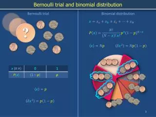
Discrete distributions. The Bernoulli distribution. The Binomial distribution. p ( x ). x. X = the number of successes in n repetitions of a Bernoulli trial p = the probability of success. The Poisson distribution. Events are occurring randomly and uniformly in time.

E N D
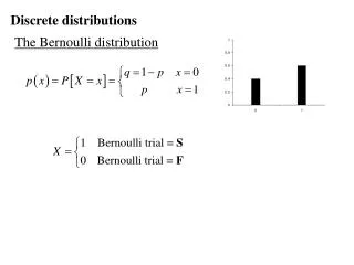
Discrete distributions The Bernoulli distribution
The Binomial distribution p(x) x X = the number of successes in n repetitions of a Bernoulli trial p = the probability of success
The Poisson distribution Events are occurring randomly and uniformly in time. X = the number of events occuring in a fixed period of time.
The Geometric distribution the Bernoulli trials are repeated independently the first success occurs (,k = 1) and X = the trial on which the 1st success occurred. P[X = x] = p(x) = p(1 – p)x – 1 = pqx – 1 The Negative Binomial distribution the Bernoulli trials are repeated independently until a fixed number, k, of successes has occurred and X = the trial on which the kth success occurred. Geometric ≡ Negative Binomial with k = 1
The Hypergeometric distribution Suppose we have a population containing N objects. The population are partitioned into two groups. • a = the number of elements in group A • b = the number of elements in the other group (group B). Note N = a+ b. • n elements are selected from the population at random. • X = the elements from group A. (n – X will be the number of elements from group B.)
Example: Hyper-geometric distribution Suppose that N = 10 automobiles have just come off the production line. Also assume that a = 3 are defective (have serious defects). Thus b = 7 are defect-free. A sample of n = 4 are selected and tested to see if they are defective. Let X = the number in the sample that are defective. Find the probability function of X. From the above discussion X will have a hyper-geometric distribution i.e.
Sampling with and without replacement Suppose we have a population containing N objects. Suppose the elements of the population are partitioned into two groups. Let a = the number of elements in group A and let b = the number of elements in the other group (group B). Note N = a+ b. Now suppose that n elements are selected from the population at random. Let X denote the elements from group A. (n – X will be the number of elements from group B.) Find the probability distribution of X. • If the sampling was done with replacement. • If the sampling was done without replacement
Solution: • If the sampling was done with replacement. Then the distribution of X is the Binomial distn.
If the sampling was done without replacement. Then the distribution of X is the hyper-geometric distn.
for large values of N, a and b Thus Thus for large values of N, a and b sampling with replacement is equivalent to sampling without replacement.
Continuousrandom variables For a continuous random variable X the probability distribution is described by the probability density function f(x), which has the following properties : • f(x) ≥ 0
Graph: Continuous Random Variableprobability density function, f(x)
Definition: A random variable , X, is said to have a Uniform distribution from a to b if X is a continuous random variable with probability density function f(x):
The Cumulative Distribution function, F(x)(Uniform Distribution from a to b)
Definition: A random variable , X, is said to have a Normal distribution with mean mand standard deviation sif X is a continuous random variable with probability density function f(x):
Graph: the Normal Distribution(mean m, standard deviation s) s m
Note: Thus the point mis an extremum point of f(x). (In this case a maximum)
Thus the points m – s, m + sare points of inflection of f(x)
Also Proof: To evaluate Make the substitution
Consider evaluating Note: Make the change to polar coordinates (R, q) z = R sin(q) and u = R cos(q)
and Hence or and Using
and or
Consider a continuous random variable, X with the following properties: • P[X ≥0] = 1, and • P[X ≥ a + b] = P[X ≥ a] P[X ≥ b] for all a > 0, b > 0. These two properties are reasonable to assume if X = lifetime of an object that doesn’t age. The second property implies:
The property: models the non-aging property i.e. Given the object has lived to age a, the probability that is lives a further b units is the same as if it was born at age a.
Let F(x) = P[X ≤ x] and G(x) = P[X ≥ x] . Since X is a continuous RV then G(x) = 1 – F(x) (P[X ≥ x] = 0 for all x.) The two properties can be written in terms of G(x): • G(0) = 1, and • G(a + b) = G(a) G(b) for all a > 0, b > 0. We can show that the only continuous function, G(x), that satisfies 1. and 2. is a exponential function
From property 2 we can conclude Using induction Hence putting a = 1. Also putting a = 1/n. Finally putting a = 1/m.
Since G(x) is continuous for all x ≥ 0. If G(1) = 0 then G(x) = 0 for all x > 0 and G(0) = 0 if G is continuous. (a contradiction) If G(1) = 1 then G(x) = 1 for all x > 0 and G() = 1 if G is continuous. (a contradiction) Thus G(1) ≠ 0, 1 and 0 < G(1) < 1 Let l = - ln(G(1)) then G(1) = e-l
To find the density of X we use: A continuous random variable with this density function is said to have the exponential distribution with parameter l.
Graphs of f(x) and F(x) f(x) F(x)
Another derivation of the Exponential distribution Consider a continuous random variable, X with the following properties: • P[X ≥0] = 1, and • P[x ≤ X ≤ x + dx|X ≥ x] = ldx for all x > 0 and small dx. These two properties are reasonable to assume if X = lifetime of an object that doesn’t age. The second property implies that if the object has lived up to time x, the chance that it dies in the small interval x to x + dx depends only on the length of that interval, dx, and not on its age x.
Determination of the distribution of X Let F (x ) = P[X ≤ x] = the cumulative distribution function of the random variable, X . Then P[X ≥0] = 1 implies that F(0) = 0. Also P[x ≤ X ≤ x + dx|X ≥ x] = ldx implies
for the unknown F. We can now solve the differential equation
Now using the fact that F(0) = 0. This shows that X has an exponential distribution with parameter l.