Download
1 / 24
240 likes | 261 Views
Terrain-following coordinates over steep and high orography. Oliver Fuhrer. Outline. Terrain-following coordinates Two idealized tests Atmosphere at rest Constant advection Possible remedy: SLEVE How to specify SLEVE parameters?. Overview.

E N D
Terrain-following coordinatesover steep and high orography Oliver Fuhrer
Outline Terrain-following coordinates Two idealized tests Atmosphere at rest Constant advection Possible remedy: SLEVE How to specify SLEVE parameters?
Overview Terrain-following coordinates have many advantages... rectangular computational mesh lower boundary condition stretching → boundary layer representation But also many disadvantages... additional terms horizontal pressure gradient formulation (Janjic, 1989) metric terms (Klemp et al., 2003) truncation error (Schär et al., 2002)
Ideal test case I • 2-dimensional • Schaer et al. MWR 2002 topography • Gal-Chen coordinates • ∆x = 1 km, Lx = 301 km • ∆z = 500 m, Lz = 22.5 km • ∆t = 25 s • Constant static stability frequency N = 0.01 s-1 • Tropopause at 11 km • Rayleight sponge (> 12 km) l2tls = .true. irunge_kutta = 1 irk_order = 3 iadv_order = 5 lsl_adv_qx = .true. lva_impl_dyn = .true. ieva_order = 3
Sensitivity: Topography height h = 0 m h = 1 m h = 3 m h = 10 m wmax = 2.8e-5 m/s wmax = 2.8e-5 m/s wmax = 2.8e-5 m/s wmax = 3.0e-5 m/s h = 30 m h = 100 m h = 300 m h = 1000 m Crash!!! wmax = 4.0e-5 m/s wmax = 0.0002 m/s wmax = 0.005 m/s wmax > 80 m/s
Ideal test case II • 2-dimensional • Schaer et al. MWR 2002 topography • Gal-Chen coordinates • ∆x = 1 kmLx = 301 km • ∆z = 500 mLz = 22.5 km • ∆t = 25 s • Constant static stability frequency N = 0.01 s-1 • Tropopause at 11 km • Rayleight sponge (> 12 km) l2tls = .true. irunge_kutta = 1 irk_order = 3 iadv_order = 5 lsl_adv_qx = .true. lva_impl_dyn = .true. ieva_order = 3
Sensitivity: Topography height h = 0 m h = 1 m h = 3 m h = 10 m wmax = 0.0001 m/s wmax = 0.001 m/s wmax = 0.002 m/s wmax = 0.007 m/s h = 30 m h = 100 m h = 300 m h = 1000 m Crash!!! wmax = 0.02 m/s wmax = 0.07 m/s wmax = 0.4 m/s wmax > 80 m/s
Explanation Advection of intensive quantity Theoretical analysis of trunction error
Upstream advection Centered advection Error term solely due to transformation Linear in h0 and u Explanation
Solution SLEVE2 zmin = 13.3 m zmin = 4.3 m zmin = 16.5 m Gal-Chen SLEVE
SLEVE2 formulation • Gal-Chen coordinate • SLEVE2 coordinate • Many parameters! How to choose?
Criteria from numerics... • Local truncation error is a function of metric terms... • ...and their derivatives
Optimal grid? • Optimize cost function • We have neglected cross-derivatives • Using n=2 for simplicity • Choose weights i inspired from SLEVE2 values
Optimize SLEVE2 • We can optimize parameters of SLEVE2 using “optimal” grid • Choose h1 like a smoothed hull of topography • Adapt decay parameters to match “optimal” grid SLEVE2 vs. Optimized
Optimize SLEVE2 • We can optimize parameters of SLEVE2 using “optimal” grid Optimized SLEVE2 SLEVE2 vs. Optimized
Conclusions COSMO shows considerable truncation errors in presence of steep and high topography Both for atmosphere at rest and constant advection test cases Better vertical coordinate transformations (SLEVE2) may reduce the amplitude at higher levels But they have many parameters to choose and effects near the land-surface can be critical Grid-optimization with numerically motivated cost function... may be a tool to choose parameters intelligently may assist in formulation of new vertical coordinates also relies on some tuning
Outlook Test optimized SLEVE2 coordinate with idealized test cases Implement optimized SLEVE2 coordinate operationally Investigate source of error for atmosphere at rest case? Behaviour of COSMO with respect to specific grid deformations could help determine weight’s of cost function Extend study to different time and space differencing scheme’s