Download

1 / 52
520 likes | 668 Views
Literature Review of Microarray Data Mining. Xin Anders March 24 th , 2006. Gene Expression. Genes are coding DNA segments which specify the composition and structure of proteins. DNA is transcribed into mRNA which in turn translates the information into proteins.

E N D
Literature Reviewof Microarray Data Mining Xin Anders March 24th, 2006
Gene Expression • Genes are coding DNA segments which specify the composition and structure of proteins. • DNA is transcribed into mRNA which in turn translates the information into proteins. • The process of transcribing DNA information into mRNA is known as gene expression. • The advances in microarray technologies revolutionized the traditional one-gene-by-one-gene approach by making it possible to study tens of thousands of genes at once.
Microarray Technologies • There are two types of microarray platforms: spotted arrays (historically called cDNA arrays) and photolithographic synthetic arrays (i.e. Affymetrix). • The fundamental difference between these two platforms lies in the experiment setups: two-dyes-labeling versus one-dye labeling and co-hybridization versus individual hybridization. • Although different data pre-processing are required for these two platforms, most downstream data analyses are similar for them. This review will focus on talking about downstream data analyses.
Spotted Arrays Figure 1. A diagram of a typical spotted arrays experiment. • Visualization of up-regulation and down regulation in one go. • No absolute gene expression levels. Source: wikipedia.com
Gene Chip (Affymetrix) Figure 2. Each gene/EST is represented by various probe sets scattered in the GeneChip. (A) Each probe is made by up to 20 couple of oligos. (B) Each probe set is made by perfect match (PM) and miss match (MM). Source: Saviozzi S. et al. 2004
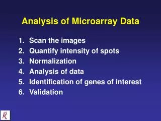
Statistical Analysis and Data Mining Techniques • Gene selection - identify differential gene expressions to a particular biological problems. • Exploratory data analysis – extract (dis)similarities of the gene expression levels (patterns) among all samples. • Discrimination analysis – train a classifier using gene expression profiles to assign any new example to a respective class. • Pathway analysis – find how genes interact as part of pathways. • Gene functional annotations – associate functional meaning to genes.
Differentially Expressed Genes • Traditionally, a fixed cut-off threshold is used to infer the increase or decrease of gene expression for a single-slide experiment. • Statistical methods based on replicate array data for ranking genes are better. • Perform an experiment as biological triplicates to increase data reliabilities (Lee ML et al. 2000, Saviozzi et al. 2004).
Statistical Tools to Rank Genes form Replicated Data • Generally, for a limited number of replicates, parametric (student t-test) or non-parametric (Mann-Whitney test) is good. • However, when multiple hypotheses are tested in the case of thousands of genes on a single microarray chip, the false positives (Type I error) can increase sharply with the number of hypotheses. a 10,000 gene array with a P value set to 0.05 ____> 10,000 * 0.05 (500) genes can be inferred even though none is differentially expressed.
Statistical Tools to Rank Genes form Replicated Data • It is often accepted to have few false positives if the majority of true positives are chosen (Leung YF 2003). • SAM (Significance Analysis of Microarrays) developed by Tusher et al. is such a technique that it uses the above concept as a tool to assist in determining a cut-off after performing adjusted t-tests.
SAM • SAM measures the strength between gene expression and the response variable (e.g. irradiated versus un-irradiated) by using repeated permutations of the data and assimilating a set of gene-specific adjusted t-tests. • The user can set the acceptable false discovery rate (FDR), significant threshold, and fold change threshold.
A SAM Example Experiment Setups: 2 states: Unirradiated (U) versus Irradiated (I) 2 biological duplicates: 1 and 2 2 technical duplicates: A and B 8 hybridizations U1A, U1B, U2A, U2B I1A, I1B, I2A, I2B Source: Tusher VG et al. 2000
A SAM Example Relative difference for the gene i is d(i) = (meanI(i) – meanU(i))/(s(i) + s0) s(i) is the standard deviation of repeated expression measurement: Genes are ranked by the magnitude of d(i) so that d(1) is the largest relative difference, d(2) is the second largest relative difference and so on. Source: Tusher VG et al. 2000
A SAM Example 8 hybridizations U1A, U1B, U2A, U2B I1A, I1B, I2A, I2B Permutations balanced on biologic duplicates are generated. U1A I1A U2A I2A U1B I1B U2B I2B … Calculate the observed relative difference d(i) Calculate dp(i) for each permutation dE(i): average over the balanced permutations Source: Tusher VG et al. 2000
A SAM Example Now we have: Observed relative difference d(i) Expected relative difference dE(i) calculated from the permutations A threshold can be chosen to yield significant genes. Source: Tusher VG et al. 2000
A SAM Example Now we have: N significant genes We want to determine the false discovery rate (FDR): 1. Horizontal cutoffs are defined as the smallest d(i) and the least negative d(i) for significantly induced and depressed respectively. 2. For each permutation, the number of false significant genes is Counted. 3. The estimated number of false significant genes F is the average Of the number of false significant genes in all permutations. 4. FDR can be calculated as F/N. Source: Tusher VG et al. 2000
SAM • SAM clearly outperforms fold test, t-test and the ANOVA based bootstrap method (Marchal K. et al 2002). • The number of permutations is affected by the number of replicates and the user should perform the full set of permutations. • Usually, a significant cutoff is chosen to give less than one false positive (Saviozzi et al. 2004).
Statistical Analysis and Data Mining Techniques • Gene selection - identify differential gene expressions to a particular biological problems. • Exploratory data analysis – extract (dis)similarities of the gene expression levels (patterns) among all samples. • Discriminant analysis – train a classifier using gene expression profiles to assign any new example to a respective class. • Pathway analysis – find how genes interact as part of pathways. • Gene functional annotations – associate functional meaning to genes.
Exploratory Data Analysis • In a more complex experiment, it is essential to extract gene expression patterns among all samples. • Exploratory data analysis, also known as unsupervised data analysis, is essentially a grouping technique that aims to find genes with similar behaviors and doesn’t require prior response measurements for the items to be grouped. • Commonly used clustering techniques include: hierachical clustering, self organization maps, k-means clustering, and principal component analysis.
Expression Matrix • To interpret the results from multiple experiments, creating an expression matrix is a common visual representation technique. • Each column of the matrix represents a single experiment and each row of the matrix represents a particular gene. Coloring the matrix provides an intuitive visual representation. Experiment 1, 2, 3 Each member is log2(ratio). If a value is 0, the color is black. A positive value is red and a negative value is green. Gene 1, 2
Before Clustering The Data • The data may need to be rescaled to prevent dominating values from obscuring other important difference. • Decide what kind of distance measurement should be used.
Hierarchical Clustering • It is an agglomerative approach in which single expression profiles are joined to form groups, which are further joined until the completion of the process. • Initially, each cluster contains a single gene. • First, the pairwise distance is calculated for all genes. • Second, two most similar genes g1 and g2 form a new cluster {g1, g2}. • Third, the distance is calculated between all other clusters and the new cluster. • Repeat step 2-3 until all objects are in one cluster.
Hierarchical Clustering • There are different methods to calculate the distances between the growing clusters and the other remaining clusters. 1. Single-linkage clustering; 2. Complete-linkage clustering; 3. Average-linkage clustering; 4. Weighted pair-group average; 5. Within-group clustering; 6. Ward’s method.
Single Linkage Clustering • The distance between two clusters i and j is calculated as the minimum distance between a member of i and a member of j. • This method tends to produce loose clusters and often result in “chaining” – a sequential addition of single samples into an existing cluster.
Complete Linkage Clustering • The distance between two clusters i and j is calculated as the greatest distance between a member of i and a member of j. • This method tends to produce compact clusters and clusters are often similar in size.
Average Linkage Clustering • The distance between clusters is calculated with average values. • There are many ways to calculate the average value. The most common one is unweighted pair-group method average (UPGMA). • In UPGMA, the distance between each point in one cluster and all points in another cluster is calculated for the average value. The two clusters with the lowest average value are joined to form a new cluster.
Average Linkage Clustering • Weighted pair-group average is identical to UPGMA except that the size of the respective cluster is used as a weight. This is useful when the cluster size is greatly varied. • Within-group clustering is similar to UPGMA except that the cluster average is used instead of all individual elements from a cluster. • Ward’s method determines whether to include a cluster by calculating the total sum of squared deviations from the mean of a cluster and joining clusters in such a way that it produces the smallest possible increase in the sum of square errors.
Hierarchical Clustering • Typically, average linkage clustering is used for gene expression data. • As clusters grow in size, the expression vector representing the cluster may no longer represent any gene in the cluster. • Furthermore, if a mistake is introduced early in the process, it can’t be corrected.
K-mean/median Clustering • K-mean/median clustering is a good alternative to hierarchical clustering if there is advanced knowledge about the number of the clusters should be represented in the data.
K-means/medians Clustering 1. Specify the fixed number (k) of clusters; 2. Randomly assign genes to clusters; 3. Calculate the mean/median expression vector for each cluster which is used to calculate the distance between clusters; 4. Shuffle genes among clusters so that each gene is now in a cluster whose mean/median expression vector is closest to that gene’s expression vector. 5. Repeat Steps 3 and 4 until genes can’t be shuffled any more.
Self-Organization Map • Self-organization map (SOM) assigns genes to a series of partition on the basis of the similarity of their expression vectors to reference vectors that are defined for each partition. • Before genes can be assigned to partitions, the user defines a geometric configuration for the partitions. Random vectors are generated for each partition and then are trained so that the data are most effectively separated.
Principal Component Analysis • Some of the data might contain redundant information. • Principal component analysis (PCA) picks out patterns in the data while reducing the effective dimensionality without significant loss of information. • PCA is difficult to be used alone but powerful when combined with another classification technique such as k-means clustering and SOM.
Statistical Analysis and Data Mining Techniques • Gene selection - identify differential gene expressions to a particular biological problems. • Exploratory data analysis – extract (dis)similarities of the gene expression levels (patterns) among all samples. • Discrimination analysis – train a classifier using gene expression profiles to assign any new sample to a respective class. • Pathway analysis – find how genes interact as part of pathways. • Gene functional annotations – associate functional meaning to genes.
Discrimination Analysis • It is also known as supervised data analysis, which trains a classifier algorithm using gene expression profiles to classify samples. • This has great promise in clinical diagnostics and has been used successfully in several recent studies.
Clinical Diagnostics with Supervised Learning T.R. Golub’s group at Whitehead Institute/MIT had several successful cases for certain cancers’ class prediction. Shipp MA et al. (2002) Diffuse large B-cell lymphoma outcome prediction by gene expression profiling and supervised machine learning. Nat. Med. 8, 68-74. Pomeroy SL et al. (2002) Prediction of central nervous system embryonal tumour outcome based on gene expression. Nature 415, 436-442.
An Example of Clinical Diagnostics Experiment setup: Known classification for Cancer1 (AML) and Cancer2 (ALL) Known samples: 27 ALL, 11 AML Affymetrix chips (6817 genes) • Find a set of informative genes whose gene expression patterns were strongly correlated with the class distinction to be predicted. • Build a classifier based on the set of informative genes. Source: T. R Golub et al. Molecular classfication of cancer: Class discovery and class prediction by gene expression monitoring. Science 286 (1999) 531-537.
An Example of Clinical Diagnostics Neighborhood analysis.
An Example of Clinical Diagnostics Class predictor.
Discrimination Analysis • The challenge for supervised data analysis is to generalize a classifier for all situations. • Over-training on the same dataset would result in over-fitting. • Different cross-validation (e.g. leave-one-out) methods can be used to establish a balance between accuracy and generalizability.
Statistical Analysis and Data Mining Techniques • Gene selection - identify differential gene expressions to a particular biological problems. • Exploratory data analysis – extract (dis)similarities of the gene expression levels (patterns) among all samples. • Discrimination analysis – train a classifier using gene expression profiles to assign any new example to a respective class. • Pathway analysis – find how genes interact as part of pathways. • Gene functional annotations – associate functional meaning to genes.
Pathway Analysis • Genes never work alone in a biological system. Analyzing microarray data in a pathway perspective can lead a higher level of understanding of the system. • A natural extension of clustering analysis: if genes are assigned to the same cluster, they may be involved in a same signal pathway. By analyzing the promoters of genes, a higher level of network may be unveiled (Pilpel Y 2001). • Various models are used to construct networks for microarray data. Bayesian network and Boolean network are two commonly used models.
A Genetic Regulatory System Source: HD Jong. Modeling and simulation of genetic regulatory systems: a literature review. J. Comp. Biol. 9 (2002) 67-103
A Simple Example of Bayesian Network A graph, conditional probability distributions for the random Variables, the joint probability distribution, and conditional Independency. Source: HD Jong. Modeling and simulation of genetic regulatory systems: a literature review. J. Comp. Biol. 9 (2002) 67-103
A Simple Example of Boolean Network For example, given a state vector 000 at t = 0, the system will move to a state 011 at the next time point t = 1 The induction of a gene is a deterministic function of the state of a group of other genes. Source: HD Jong. Modeling and simulation of genetic regulatory systems: a literature review. J. Comp. Biol. 9 (2002) 67-103
Pathway Analysis • A free software called Pathway Processor developed by the Bauer Center for Genomics at Harvard can map expression data onto metabolic pathways and evaluate which metabolic pathways are most affected. Fisher Exact test is used to score pathways according to the probability that as many or more genes in a pathway would be altered in a given experiment than by chance alone.
Statistical Analysis and Data Mining Techniques • Gene selection - identify differential gene expressions to a particular biological problems. • Exploratory data analysis – extract (dis)similarities of the gene expression levels (patterns) among all samples. • Discrimination analysis – train a classifier using gene expression profiles to assign any new example to a respective class. • Pathway analysis – find how genes interact as part of pathways. • Gene functional annotations – associate functional meaning to genes.
Gene Functional Annotation • In order to know whether some specific biological process is strongly affected by transcriptional expression, we have to associate functional meaning to genes by using gene functional annotations. • Researchers rely on robust gene annotations to link functional to transcriptional profiling. • Gene Ontology (GO) is a commonly used control vocabulary for describing the roles of genes and gene products in any organism.
Gene Ontology • GO is divided into three categories: molecular function, biological process, and cellular component. [Term] id: GO:0000786 name: nucleosome namespace: cellular_component def: "A complex comprised of DNA wound around a multisubunit core and associated proteins, which forms the primary packing unit of DNA into higher order structures." [GOC:elh] is_a: GO:0043234 ! protein complex relationship: part_of GO:0000785 ! chromatin
Gene Ontology • GO terms are organized in directed acyclic graphs, which differ from hierarchies in that a child term can have many parent terms. Monosaccharide biosynthesis Hexose metabolism Hexose biosynthesis
Gene Ontology • GO terms become associated with their appropriate gene products through collaborating databases. These databases annotate genes with GO terms, providing references and indicating what kind of evidence is available to support the annotations.
References • Aas Km(2001). Microarray data mining: a survey. Norsk Regnesentral: Norwegian Computing Center. • Dudoit S. et al. (2000). Comparison of discrimination methods for the classification of tumors using gene expression data. Technical report no. 576, University of Claifornia, Berkely. • Saviozzi S. et al. (2004). Microarray data analysis and mining. Methods Mol. Med, 94: 67-89. • Lee ML et al. (2000). Importance of replication in microarray gene expression studies: statistical methods and evidence from repetitive cDNA hybridizations. Proc. Natl. Acad. Sci. USA, 97: 9834-39. • Leung YF and Cavalieri D (2003). Fundamentals of cDNA microarray data analysis. Trends Genet., 19(11): 649-59. • Tusher VG et al. (2001). Significance analysis of microarrays applied to ionizing radiation response. Proc. Natl. Acad. Sci. USA, 98: 5116-21. • Marchal K et al. (2002). Comparison of different methodologies to identify differentially expressed genes in two-example cDNA microarrays. J. Bio Systems, 10: 409-430. • Eisen MB et al. (1998).Cluster Analysis and display of genome-wide expression patterns. Proc. Natl. Acad. Sci. USA, 96: 2907-2912.