Mining for Low-abundance Transcripts in Microarray Data
Mining for Low-abundance Transcripts in Microarray Data. Yi Lin 1 , Samuel T. Nadler 2 , Alan D. Attie 2 , Brian S. Yandell 1,3 1 Statistics, 2 Biochemistry, 3 Horticulture, University of Wisconsin-Madison September 2000. Basic Idea.

Mining for Low-abundance Transcripts in Microarray Data
E N D
Presentation Transcript
Miningfor Low-abundance Transcriptsin Microarray Data Yi Lin1, Samuel T. Nadler2, Alan D. Attie2, Brian S. Yandell1,3 1Statistics, 2Biochemistry, 3Horticulture, University of Wisconsin-Madison September 2000
Basic Idea • DNA microarrays present tremendous opportunities to understand complex processes • Transcription factors and receptors expressed at low levels, missed by most other methods • Analyze low expression genes with normal scores • Robustly adapt to changing variability across average expression levels • Basis for clustering and other exploratory methods • Data-driven p-value sensitive to low abundance & changes in variability with gene expression
DNA Microarrays • 100-100,000 items per “chip” • cDNA, oligonucleotides, proteins • dozens of technologies, changing rapidly • expose live tissue from organism • mRNA cDNA hybridize with chip • read expression “signal” as intensity (fluorescence) • design considerations • compare conditions across or within chips • worry about image capture of signal
Low Abundance Genes • background adjustment • remove local “geography” • comparing within and between chips • negative values after adjustment • low abundance genes • virtually absent in one condition • could be important genes: transcription factors, receptors • large measurement variability • early technology (bleeding edge) • prevalence across genes on a chip • 0-20% per chip • 10-50% across multiple conditions
Log Transformation? • tremendous scale range in mean intensities • 100-1000 fold common • concentrations of chemicals (pH) • fold changes have intuitive appeal • looks pretty good in practice • want transformed data to be roughly normal • easy to test if no difference across conditions • looking for genes that are “outliers” • beyond edge of bell shaped curve • provide formal or informal thresholds
Exploratory Methods • Clustering methods (Eisen 1998, Golub 1999) • Self-organizing maps (Tamayo 1999) • search for genes with similar changes across conditions • do not determine significance of changes in expression • require extensive pre-filtering to eliminate • low intensity • modest fold changes • may detect patterns unrelated to fold change • comparison of discrimination methods (Dudoit 2000)
Confirmatory Methods • ratio-based decisions for 2 conditions (Chen 1997) • constant variance of ratio on log scale, use normality • anova (Kerr 2000, Dudoit 2000) • handles multiple conditions in anova model • constant variance on log scale, use normality • Bayesian inference (Newton 2000, Tsodikov 2000) • Gamma-Gamma model • variance proportional to squared intensity • error model (Roberts 2000, Hughes 2000) • variance proportional to squared intensity • transform to log scale, use normality
0. acquire data Q, B 7. standardize Z=Y –center spread 1. adjust for background A=Q – B 6. center & spread 2. rank order genes R=rank(A)/(n+1) Y = contrast 3. normal scores N=qnorm(R) X = mean 5. mean intensity X=mean(N) 4. contrast conditions Y=N1 –N2
Normal Scores Procedure adjusted expression A = Q – B rank order R = rank(A) / (n+1) normal scores N = qnorm( R ) average intensity X = (N1+N2)/2 difference Y = N1 – N2 variance Var(Y | X) 2(X) standardization S = [Y –(X)]/(X)
Motivate Normal Scores • natural transformation to normality is log(A) • background intensity B = bd +B • measured with error • attenuation d may depend on condition • gene measurement Q = [exp(g+h+)+b]d+Q • gene signal g • degree of hybridization h: • intrinsic noise (variance may depend on g) • attenuation (depends thickness of sample, etc.) • subtract background: A = Q – B • adjusted measurements A = dexp(g+h+)+ • symmetric measurement error =B –Q
Motivate Normal Scores (cont.) • adjusted measurements: A = Q – B = dG+ • log expression level: log(G) = g+h+ • gene signalg confounded with hybridization h • unless hybridization h independent of condition • G is observed if • no measurement error • no dye or array effect (no attenuation d) • no background intensity • natural under this model to consider N=log(G) • normal scores almost as good
Robust Center & Spread • genes sorted based on X • partitioned into many (about 400) slices • containing roughly the same number of genes • slices summarized by median and MAD • MAD = median absolute deviation • robust to outliers (e.g. changing genes) • MAD ~ same distribution across X up to scale • MADi = i Zi, Zi ~ Z, i = 1,…,400 • log(MADi ) = log(i) + log(Zi) • median ~ same idea
Robust Center & Spread • MAD ~ same distribution across X up to scale • log(MADi ) = log(i) + log(Zi), I = 1,…,400 • regress log(MADi) on Xi with smoothing splines • smoothing parameter tuned automatically • generalized cross validation (Wahba 1990) • globally rescale anti-log of smooth curve • Var(Y|X) 2(X) • can force 2(X) to be decreasing • similar idea for median • E(Y|X) (X)
Motivation for Spread • log expression level: log(G) = g+h+ • hybridization h negligible or same across conditions • intrinsic noise may depend on gene signal g • compare two conditions 1 and 2 • Y = N1 – N2 log(G1) – log(G2) = g1 –g2+ 1 -2 • no differential expression: g1=g2=g • Var(Y|g) = 2(g) • gX suggests condition on X instead, but: • Var(Y | X) not exactly 2(X) • cannot be determined without further assumptions
Simulation of Spread Recovery • 10,000 genes: log expression Normal(4,2) • 5% altered genes: add Normal(0,2) • no measurement error, attenuation • estimate robust spread
Bonferroni-corrected p-values • standardized normal scores • S = [Y –(X)]/(X) ~ Normal(0,1) ? • genes with differential expression more dispersed • Zidak version of Bonferroni correction • p = 1 – (1 – p1)n • 13,000 genes with an overall level p = 0.05 • each gene should be tested at level 1.95*10-6 • differential expression if S > 4.62 • differential expression if |Y –(X)| > 4.62(X) • too conservative? weight by X? • Dudoit (2000)
Simulation Study • simulations with two conditions • 10,000 genes • g1 ,g2 ~ Normal(4,2) for nonchanging genes • 5% with differential expression • gc ~ Normal(4,2) + Normal(3-rank(X)/(n+1),1/2) • up- or down-regulated with probability 1/2 • intrinsic noise ~ Normal(0,0.5) • attenuation = 1 • measurement error variance= 0, 1, 2, 5, 10, 20
Comparison of Methods • differential expression for two conditions • Newton (2000) J Comp Biol • Gamma-Gamma-Bernouli model • Bayesian odds of differential expression • Chen (1997) • constant ratio of expressions • underlying log-normality • normal scores (Lin 2000) • some (unknown) transformation to normality • robust, smooth estimate of spread & center • Bonferroni-style p-values
Comparison with E. coli Data • 4,000+ genes (whole genome) • Newton (2000) J Comp Biol • Bayesian odds of differential expression • IPTG-b known to affect only a few genes • ~150 genes at low abundance • including key genes
Diabetes & Obesity Study • 13,000+ gene fragments (11,000+ genes) • oligonuleotides, Affymetrix gene chips • mean(PM) - mean(NM) adjusted expression levels • six conditions in 2x3 factorial • lean vs. obese • B6, F1, BTBR mouse genotype • adipose tissue • influence whole-body fuel partitioning • might be aberrant in obese and/or diabetic subjects • Nadler (2000) PNAS
Low Abundance Obesity Genes • low mean expression on at least 1 of 6 conditions • negative adjusted values • ignored by clustering routines • transcription factors • I-kB modulates transcription - inflammatory processes • RXR nuclear hormone receptor - forms heterodimers with several nuclear hormone receptors • regulation proteins • protein kinase A • glycogen synthase kinase-3 • roughly 100 genes • 90 new since Nadler (2000) PNAS
Microarray ANOVAs • Kerr (2000) • gene by condition interaction • Nijk = genei + conditionj + gene*conditionij + rep errorijk • conditions organized in factorial design • experimental units may be whole or part of array • genes are random effects • focus on outliers (BLUPs), not variance components • gene*conditionij = differential expression • allow variance to depend on genei main effect • replication to improve precision, catch gross errors
Microarray Random Effects • variance component for non-changing genes • robust estimate of MS(G*C) using smoothed MAD • rescale normal score response N by spread (X) • look for differential expression • or use clustering methods • variance component for replication • robust estimate of MSE using smoothed MAD • look for outliers = gross errors
Microarray QTLs • condition may be genotype • whole organism or pattern of genes • genotype may be inferred rather than known exactly • Nijk = genei + QTLj + gene*QTLij + individualijk • QTL genotype depends on flanking markers • mixture model across possible QTL genotypes • single vs. multiple QTL • single QTL may influence numerous genes • epistasis = inter-genic interaction • modification of biochemical pathway(s)