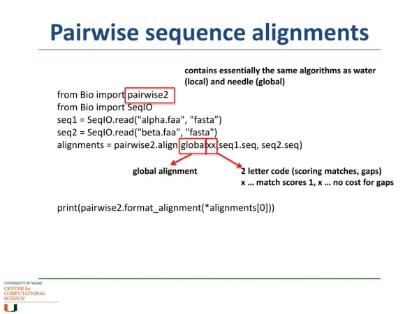
Pairwise Sequence Comparison

1. Pairwise Sequence Comparison Stat 246, Spring 2002, Week 5,

2. Sequence comparison: topics • General concepts • Dot plots • Global alignments • Scoring matrices • Gap penalties • Dynamic programming • Chance or common ancestry?

3. Dot Plot • This is the earliest, simplest and most complete method for comparing two sequences • It is possible to filter the plot to minimise noise whilst preserving the obvious relationship • This plot can identify • regions of similarity • internal repeats • rearrangement events

4. (Add a “guard” row and colum.) Sequence 2 along: b A C A C A C T A Sequence 1 down: . a A A dot goes where the two sequences match G C A Connect the dots along diagonals. C A C A

5. Extensions to dot plots • Modern dot plots are more sophisticated, using the notions of • window : size of diagonal strip centered on an entry, over which matching is accumulated, and • stringency: the extent of agreement required over the window, before a dot is placed at the central entry. • e.g. for a window of size 5, we might require at least 3 matches, and then we put a dot in the central spot. More complex scoring rules can be used.

6. Human  globin vs. human myoglobin

7. Human LDL receptor vs. itself (w=30, s=9)

8. 0 200 400 600 800 800 600 400 200 0 ldlrecep.pep ck: 3,641, 1 to 860 COMPARE Window: 40 Stringency: 15.0 Points: 5,287 ldlrecep.pep ck: 3,641, 1 to 860 Human LDL receptor vs. itself (40, 15)

9. 0 200 400 600 800 800 600 400 200 0 ldlrecep.pep ck: 3,641, 1 to 860 COMPARE Window: 40 Stringency: 17.5 Points: 3,079 ldlrecep.pep ck: 3,641, 1 to 860 Human LDL receptor vs. itself (40, 17.5)

10. 0 200 400 600 800 800 600 400 200 0 ldlrecep.pep ck: 3,641, 1 to 860 COMPARE Window: 40 Stringency: 20.0 Points: 2,295 ldlrecep.pep ck: 3,641, 1 to 860 Human LDL receptor vs. itself (40, 20)

11. Plasmodium falciparum MSP3 vs. itself (30,9)

12. 0 100 200 300 300 200 100 0 msp3.pep ck: 4,247, 1 to 380 COMPARE Window: 20 Stringency: 9.0 Points: 15,619 msp3.pep ck: 4,247, 1 to 380 Plasmodium falciparum MSP3 vs. itself (20,9)

13. 0 100 200 300 300 200 100 0 msp3.pep ck: 4,247, 1 to 380 COMPARE Window: 10 Stringency: 9.0 Points: 1,263 msp3.pep ck: 4,247, 1 to 380 Plasmodium falciparum MSP3 vs. itself (10,9)

14. Global alignment An alignment of two sequences a and b is an arrangement of a and b by position, where a and b can be padded with gap symbols to achieve the same length: a: AGCACAC-A or AG-CACACA b: A-CACACTA ACACACT-A If we read the alignment column-wise, we have a protocol of edit operations that lead from a to b. Left: Match (A,A) Right: Match (A,A) Delete (G,-) Replace (G,C) Match (C,C) Insert (-,A) Match (A,A) Match (C,C) Match (C,C) Match (A,A) Match (A,A) Match (C,C) Match (C,C) Replace (A,T) Insert (-,T) Delete (C,-) Match (A,A) Match (A,A) The left-hand alignment shows one Delete, one Insert, and the other edit operations are Matches. The right-hand alignment shows one Insert, one Delete, two Replaces, and some trivial ones.

15. Next we turn the edit protocol into a measure of distance by assigning a “cost” or “weight” S to each operation. For example, for arbitrary characters u,v from A we may define S(u,u) = 0; S(u,v) = 1 for u ≠ v; S(u,-) = S(-,v) = 1. (Unit Cost) This scheme is known as the Levenshtein distance, also called unit cost model. Its predominant virtue is its simplicity. In general, more sophisticated cost models must be used. For example, replacing an amino acid by a biochemically similar one should weight less than a replacement by an amino acid with totally different properties. Details shortly. Now we are ready to define the most important notion for sequence analysis: The cost of an alignment of two sequences a and b is the sum of the costs of all the edit operations that lead from a to b. An optimal alignment of a and b is an alignment which has minimal cost among all possible alignments. The edit distance of a and b is the cost of an optimal alignment of a and b under a cost function S. We denote it by d(a,b). Using the unit cost model for S in our previous example, we obtain the following cost: a: AGCACAC-A or AG-CACACA b: A-CACACTA ACACACT-A cost: 2 cost: 4 Here it is easily seen that the left-hand assignment is optimal under the unit cost model, and hence the edit distance d(a,b) = 2. Cost (scoring) of global alignments; optimal global alignments

16. More general scores = - costs: see later. 134 LQQGELDLVMTSDILPRSELHYSPMFDFEVRLVLAPDHPLASKTQITPEDLASETLLI | ||| | | |||||| | || || 137 LDSNSVDLVLMGVPPRNVEVEAEAFMDNPLVVIAPPDHPLAGERAISLARLAEETFVM D:D = +6 D:R = -2 From Henikoff 1996

17. Scoring Matrices • Physical/Chemical similarities • comparing two sequences according to the properties of their residues may highlight regions of structural similarity • Identity matrices • by stressing only identities in the alignment, stretches of sequence that may have diverged will not penalise any remaining common features

18. Scoring Matrices (ctd) • As the direct source of residue by residue comparison scores the scoring matrix you choose will have a major impact on the alignment calculated • The most commonly used will be one of the mutation matrices • PAM or BLOSUM • Von Bing will explain the derivation of these and other mutation matrices next Tuesday. • The matrix that performs best will be the matrix that best reflects the evolutionary separation of the sequences being aligned.

19. AGCTGATCA... AACCGGTTA... Alignment: Hypotheses: H = homologous (indep. sites, Jukes-Cantor) R = random (indep. sites, equal freq.) Statistical motivation for alignment scores pr(data|H) = pr( |H) = pr( |H) x ... = (1-p)apd d = # disagreements, a = # agreements, p = (1-e-8at) pr(data|R) = pr( |R) = pr( |R) x ... = ( )a( )d = a  log + d  log . Since p < , log <0, log >0 score = a s + d  (-m) s >0 match score, -m <0 mismatch penalty Note that if at 0, p 6at, 1-p 1 and so s log4, while -m log8at is large and negative: a big difference in the two scores. Conversely, if at is large, p = (1-e), = 1-e, and m = log(1-e) -e, while 1-p = (1+3e), = 1+3e, and so s = log(1+3e) 3e. Thus the scores are about 3:1. AA GA AA GA

20. a gap free alignment of two a.a. sequence fragments a1 ..... am b1 ..... bm data = We can do the same with any other Markov substitution matrix for molecular evolution. E.g. with a PAM or BLOSUM matrix of probabilities, m P 1 P i pr(data|H) = paipaibi(2t) pr(data|R) = paipbi log{} = log{ } paibi(2t)/ pbi S i The elements of a log-odds score matrix are typically > 0 on the diagonal and < 0 off the diagonal, but not always. Also the relative sizes of match and mismatch penalties increase as #PAMs (t) decreases. Thus PAM(120) is more stringent than PAM(250), while PAM(360) is less stringent than it. PAM(0) = the identity matrix is the toughest. There are plenty of score matrices based on other principles.

21. Below diagonal: BLOSUM62 substitution matrixAbove diagonal: Difference matrix obtained by subracting the PAM 160 matrix entrywise.From Henikoff & Henikoff 1992

22. Above diagonal: SG scoring system (Feng et al., 1985) Below diagonal: Log-odds matrix for 250 PAMs (Dayhoff et al., 1978)

23. Gap penalties • Gap penalties are usually composed of two parts: • Gap opening penalty • This reduces the alignment score and therefore must create more significant alignment downstream than would be present if no gap were created • The size of the penalty is usually of the order of one to three times the size of values in the scoring matrix

24. Gap penalties (ctd) • Gap extension penalty • If a gap has been created then extending it should not be as hard to do • On the other hand we want to limit the size of the gap to practical lengths • A smaller gap extension penalty may allow an alignment to resolve situations where complete loops may be missing between one structure and another

25. eclustalw May 24, 1999 18:44 lgb1_pea.pep ck: 2970 from: 1 to: 147 Length: 147 hbhu.pep ck: 3588 from: 1 to: 147 Length: 147 Pairwise similarity parameter: K-Tuple length: 1 Gap Penalty: 3 Number of diagonals: 5 Diagonal window size: 5 Scoring Method: Percentage Multiple alignment parameter: Gap Penalty (fixed): 1.00 Gap Penalty (varying): 0.05 Gap separation penalty range: 8 Percent. identity for delay: 40% List of hydrophilic residue: GPSNDQEKR Protein Weight Matrix: blosum 10 20 30 40 50 60 . . . . . . LGB1_PEA.pep --GFTDKQE-ALVNSSSEFKQNLPGYSILFYTIVLEKAPAAKGLF-SF--LKDTAGVEDS HBHU.pep MVHLTPEEKSAVTALWGKVNVDEVGGEALGRLLVVY--PWTQRFFESFGDLSTPDAVMGN * . *. * * .*. * .. * ** * * LGB1_PEA.pep PKLQAHAEQVFGLVRDSAAQLR-TKGEVVLGNATLGAIHVQKGVTNP-HFVVVKEALLQT HBHU.pep PKVKAHGKKVLGAFSDGLAHLDNLKGTF----ATLSELHCDKLHVDPENFRLLGNVLVCV **..** .* * * *.* ** *** .* * * .* .. *. LGB1_PEA.pep IKKASGNNWSEELNTAWEVAYDGLATAIKKAMKTA HBHU.pep LAHHFGKEFTPPVQAAYQKVVAGVANAL--AHKYH . . * . ...* . *.*.*. * * Low gap penalty

26. Middling gap penalty eclustalw May 24, 1999 18:50 lgb1_pea.pep ck: 2970 from: 1 to: 147 Length: 147 hbhu.pep ck: 3588 from: 1 to: 147 Length: 147 Pairwise similarity parameter: K-Tuple length: 1 Gap Penalty: 3 Number of diagonals: 5 Diagonal window size: 5 Scoring Method: Percentage Multiple alignment parameter: Gap Penalty (fixed): 25.00 Gap Penalty (varying): 0.05 Gap separation penalty range: 8 Percent. identity for delay: 40% List of hydrophilic residue: GPSNDQEKR Protein Weight Matrix: blosum 10 20 30 40 50 60 . . . . . . LGB1_PEA.pep ----GFTDKQEALVNSSSEFKQNLPGYSILFYTIVLEKAPAAKGLFSFLKDTAGVEDSPK HBHU.pep MVHLTPEEKSAVTALWGKVNVDEVGGEALGRLLVVYPWTQRFFESFGDLSTPDAVMGNPK .* . * .. .* . * * * ** LGB1_PEA.pep LQAHAEQVFGLVRDSAAQLRTKGEVVLGNATLGAIHVQKGVTNP-HFVVVKEALLQTIKK HBHU.pep VKAHGKKVLGAFSDGLAHLDN---LKGTFATLSELHCDKLHVDPENFRLLGNVLVCVLAH ..** .* * * *.* . . *** .* * * .* .. *. . . LGB1_PEA.pep ASGNNWSEELNTAWEVAYDGLATAIKKAMKTA HBHU.pep HFGKEFTPPVQAAYQKVVAGVANALAHKYH-- * . ...* . *.*.*. . .

27. eclustalw May 24, 1999 18:52 lgb1_pea.pep ck: 2970 from: 1 to: 147 Length: 147 hbhu.pep ck: 3588 from: 1 to: 147 Length: 147 Pairwise similarity parameter: K-Tuple length: 1 Gap Penalty: 3 Number of diagonals: 5 Diagonal window size: 5 Scoring Method: Percentage Multiple alignment parameter: Gap Penalty (fixed): 50.00 Gap Penalty (varying): 0.05 Gap separation penalty range: 8 Percent. identity for delay: 40% List of hydrophilic residue: GPSNDQEKR Protein Weight Matrix: blosum 10 20 30 40 50 60 . . . . . . LGB1_PEA.pep ----GFTDKQEALVNSSSEFKQNLPGYSILFYTIVLEKAPAAKGLFSFLKDTAGVEDSPK HBHU.pep MVHLTPEEKSAVTALWGKVNVDEVGGEALGRLLVVYPWTQRFFESFGDLSTPDAVMGNPK .* . * .. .* . * * * ** LGB1_PEA.pep LQAHAEQVFGLVRDSAAQLRTKGEVVLGNATLGAIHVQKGVTNPHFVVVKEALLQTIKKA HBHU.pep VKAHGKKVLGAFSDGLAHLDNLKGTFATLSELHCDKLHVDPEN--FRLLGNVLVCVLAHH ..** .* * * *.* . . * . ... * * .. *. . . LGB1_PEA.pep SGNNWSEELNTAWEVAYDGLATAIKKAMKTA HBHU.pep FGKEFTPPVQAAYQKVVAGVANALAHKYH-- * . ...* . *.*.*. . . Very high gap penalty

28. Dynamic Programming For obtaining optimal alignments This is a mathematical implementation that can be seen as an extension of the dotplot method Rather than dots, the comparison matrix positions are assigned values that reflect the scores in the scoring matrix

29. Dynamic Programming The optimum alignment is obtained by tracing the highest scoring path from the top left-hand corner to the bottom right-hand corner of the matrix When the alignment steps away from the diagonal this implies an insertion or deletion event, the impact of which can be assessed by the application of a gap penalty

30. b A C A C A C T A a A 0 1 0 1 0 1 1 0 G 1 1 1 1 1 1 1 1 C 1 0 1 0 1 0 1 1 A 0 1 0 1 0 1 1 0 C 1 0 1 0 1 0 1 1 A 0 1 0 1 0 1 1 0 C 1 0 1 0 1 0 1 1 A 0 1 0 1 0 1 1 0

31. Dynamic programming: the formula Suppose that our two sequences are a=(a1,...,am) and b=(b1,...,bn), and that we denote by dij the edit distance between the initial segmentsai=(a1,...,ai) and bj=(b1,...,bj) of a and b. Extend this to i=j=0 by writing d00=0. Supposing that a deletion or an insertion incurs a penalty of +1, the following formula summarizes our verbal argument: dij=min(di-1,j-1 + s(ai,bj), di,j-1 + 1, di-1,j + 1). (More is needed to give a complete algorithm: what is it?)

32. b A C A C A C T A 0 1 2 3 4 5 6 7 8 a A 1 0 1 2 3 4 5 6 7 G 2 1 1 2 3 4 5 6 7 C 3 2 1 2 2 3 4 5 6 A 4 3 2 1 2 2 3 4 5 C 5 4 3 2 1 2 2 3 4 A 6 5 4 3 2 1 2 3 3 C 7 6 5 4 3 2 1 2 3 A 8 7 6 5 4 3 2 2 2

33. Chance or common ancestry? Idea: calculate optimal alignment scores for pairs of sequences where one is a randomized (shuffled) version of the original. This will give a distribution of random scores, representing chance similarity rather than homology. The score from our original pair of sequences can be referred to this distribution and assigned a Z-score (subtract mean of randoms and divide by SD of randoms), or (better) a p-value. Criticism: Such random a.a. sequences might have plausible a.a. compositions but are quite unlike real protein sequences. Partial reply: a) restrict the randomization to blocks; or, b) create a distribution of chance similarity scores using real a.a. sequences known or assumed not to be homologous to our query sequence. [Other approaches use theory, but this is still subject to the criticism above.]

34. Dynamic ProgrammingBased on notes by George Rudy, formerly WEHI.

35. “Life must be lived forwards and understood backwards.” Søren Kierkegaard

36. What is DP? Operations research: “A mathematical formalism applicable to problems involving optimization of decisions over time.” (after R. Bellman and S. Dreyfus) Bioinformatics : “An algorithm for finding optimal sequence alignments given an additive alignment score.” ( after R. Durbin, et al.) Computer programming: “An approach to algorithm design whereby the target problem is decomposed into smaller problems that are then solved independently.” (after R. Sedgewick)

37. Where did DP come from? - Richard Bellman - The RAND Corporation - “Dynamic” and “Programming”

38. Where can DP be applied? - Both discrete and continuous problems concerning deterministic, stochastic, or adaptive processes - Multiple fields: research, industry, finance,… - Examples: allocation processes smoothing and scheduling processes optimal search and stopping techniques optimal trajectories multistage production processes feedback control processes Markovian decision processes

39. DP in biomedical literature (1)

40. DP in biomedical literature (2) - A symmetric-iterated multiple alignment of protein sequences. [Brocchieri, L. and Karlin S., J. Mol. Biol. 276(1):249-64, 1998.] - Sequence assembly validation by multiple restriction digest fragment coverage analysis. [Rouchka, E.C. and States, D.J., ISMB. 6:140-7, 1998.] - Automated protein sequence database classification. I. Integration of compositional similarity search, local similarity search, and multiple sequence alignment. [Gracy, J. and Argos, P., Bioinformatics 14(2):164-73, 1998.] - A segment-based dynamic programming algorithm for predicting gene structure. [Wu, T.D., J. Comput. Biol. 3(3):375-94, 1996.] - Automatic detection of cardiac contours on MR images using fuzzy logic and dynamic programming. [Lalande A. et al., Proc. AMIA Annu. Fall Symp. :474-8, 1997.] - Process models for production of beta-lactam antibiotics. [Bellgardt, K.H., Adv. Biochem. Eng. Biotechnol. 60:153-94, 1998.] - Dynamic programming approach for newborn’s incubator humidity control. [Bouattoura, D. et al., IEEE Trans. Biomed. Eng. 45(1):48-55, 1998.] - Minimum energy trajectories of the swing ankle when stepping over obstacles of different heights. [Chou L.S. et al., J. Biomech. 30(2):115-20, 1997.] - A theoretical study of the socioecology of ungulates. II. A dynamic programming study of the stochastic formulation. [Paveri-Fontana, S.L. and Focardi, S. Theor. Popul. Biol. 46(3):279-99, 1994.]

41. What problems are suitable for DP? - Essential components (common to all OR problems): a decision-maker access to results of decisions - Additionally: decisions are sequential later decisions are affected by earlier ones effect of a decision can be calculated independently of other decisions

42. The Stagecoach Problem (1) H 2 3 E L 5 1 3 5 C I O 4 1 4 1 2 2 F M A B 7 2 2 8 1 0 P D J 3 5 2 4 G N 4 2 K [after S. E. Dreyfus]

43. Some terminology - Vertex - Edge - Path -Monotonic-to-the-right - (Admissible) path - Stage - State

44. The Stagecoach Problem (2) H 2 3 E L 5 1 3 5 C I O 4 1 4 1 2 2 F M A 0 B 7 2 2 8 1 0 P D J 3 5 2 4 G N 4 2 K

45. The Stagecoach Problem (2) H 2 3 E L 5 1 3 5 C I O 4 2 1 4 1 2 2 F M A 0 B 7 2 2 8 1 0 P D J 1 3 5 2 4 G N 4 2 K

46. The Stagecoach Problem (2) H 2 3 E L 5 1 3 5 C I O 4 2 1 4 1 2 2 F M A 0 B 4 7 2 2 8 1 0 P D J 1 3 5 2 4 G N 4 2 K

47. The Stagecoach Problem (2) H 10 2 3 E L 7 5 1 3 5 C I O 8 4 2 1 4 1 2 2 F M A 0 B 4 7 2 2 8 1 0 P D J 1 6 3 5 2 4 G N 5 4 2 7 K

48. The Stagecoach Problem (2) H 10 2 3 E L 9 7 5 1 3 5 C I O 12 8 4 2 1 4 1 2 2 F M A 13 0 B 8 4 7 2 2 8 1 0 P D J 14 1 6 3 5 2 4 G N 11 5 4 2 7 K

49. Some more terminology - Optimal value function - Policy - Optimal policy function

50. The Stagecoach Problem (3) H 10 2 3 E L 9 7 5 1 3 5 C I O 12 8 4 2 1 4 1 2 2 F M A 13 0 B 8 4 7 2 2 8 1 0 D J P 14 1 6 3 5 2 4 G N 11 5 4 2 7 K