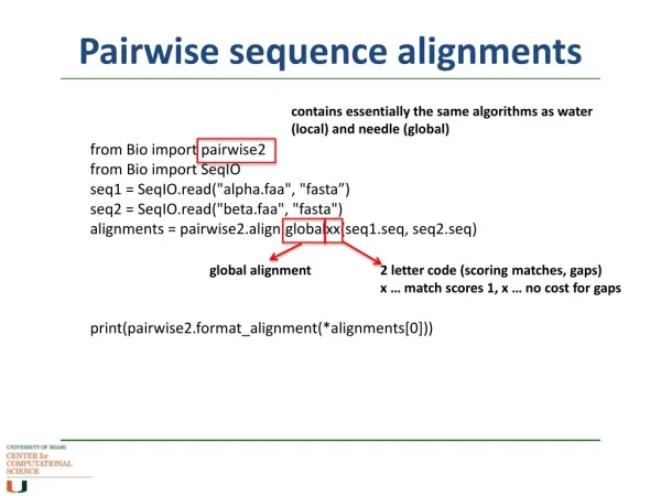
Pairwise sequence alignments

1. Pairwise sequence alignments • Dynamic programming (Needleman-Wunsch), finds optimal alignment • Heuristics: Blast (Altschul et al) does not guarantee finding optimal alignment, but fast

2. Pairwise sequence alignments APLFVA----ITRSDD APVFIAGDTRITRSEE Assumptions: • evolution of sequences through mutations and deletions/insertions; • the closer similarity between sequences, the more chances they are evolutionarily related.

3. Similarity measures: Percent Identity Identity score – Exact matches receive score of 1 and non-exact matches score of 0 AVLILKQW AVLI I LQ T ------------------------------ 1 1 1 1 0 0 1 0 = 5 (Score of the alignment under “identity”) Percent identity:identity_score/length_of_the_shorter_protein Disadvantage of % id: does not take into account the similarity between their properties.

4. Substitution Matrices – measure of “similarity” score of amino-acids • M(i,j) ~ probability of substituting i into j over some time period • Percent Accepted Mutation (PAM) unit = evolutionary time corresponding to average of 1 mutation per 100 res. • Two most popular classes of matrices: • PAMn: relates to mutation probabilities in evolutionary interval of n PAM units (PAM 120 is often used in practice) • BLOSUMx: relates to mutation probabilities observed between pairs of related proteins that diverged so above x % identity. BLOSUM62 ~ PAM250

5. Scoring the gaps The two alignments below have the same score. The second alignment is better. Solution: Have additional penalty for opening a gap ATTTTAGTAC ATT- - AGTAC ATTTTAGTAC A-T-T -AGTAC Affine gap penalty w(k) = h + gk ; h,g constants Interpretation: const of starting a gap: h+g, extending gap: +g

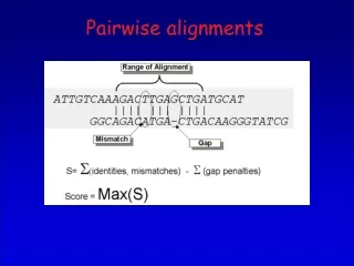
6. Dot plot illustration Adapted from T. Przytycka The alignment corresponds to path from upper left corner to lower right corner going trough max. nr of dots Deletions TTACTCAAT - - - - - ACTCA- TTAC

7. Gap penalties Consider two pairs of alignments: ATCG ATTG AT – C G AT T - G They have the same score but the right alignment is more likely from evolutionary perspective (simpler explanation = better explanation) and • First problem is corrected by introducing “gap penalty”: for each gap subtract gap penalty from the score • Second problem is corrected by introducing additional penalty for opening a gap: and AT - C - T A AT T T T TA ATC - - T A ATT T T TA Affine gap penalty w(k) = h + gk ; h,g constants Interpretation: const of starting a gap: h+g, extending gap: +g

8. Organizing the computation – dynamic programming table Align j Align(i,j) = Align(Si,S’j)= max i { Align(Si-1,S’j-1)+s(ai, a’j) Align(Si-1,S’j) - g Align(Si,S’j-1) - g +s(ai,aj) max

9. Recovering the path A T T G A T T G - A T - G C A T G C

10. Ignoring initial and final gaps – semiglobal comparison CAGCA - CTTGGATTCTCGG - - - CAGCGTGG - - - - - - - - No penalties for these gaps Recall the initialization step for the dynamic programming table: A[0,i], A[j,0]– these are responsible for initial gaps. set them to zero! How to ignore final gaps? Take the largest value in the last row /column and trace-back form there

11. Comparing similar sequences Similar sequences – optimal alignment has small number of gaps. The “alignment path” stays close to the diagonal From book Setubal Meidanis”Introduction Comp. Mol. Biol”

12. Local and global alignments Global Local

13. Local alignment (Smith - Waterman) So far we have been dealing with global alignment. Local alignment – alignment between substrings. Main idea: If alignment becomes too bad – drop it. a[i-1,j-1]+ s(ai, aj) a[i-1,j +g a[i,j-1]+ g 0 { a[i,j]= max

14. Example

15. BLAST • Local heuristics • Fast • Good statistics • Precalculated lookup table of all high score word matches of three residue long • Extend the hit until score drops below some threshold

16. Sequence-profile alignments: sequence profiles describe conserved features with respect to position in multiple alignment 1 2 3 4 5 6 7 IDVVVVC --------------------------------------- LDLV--C A 2 -2 -2 -1 -1 -1 -2 LDLVFVC --------------------------------------- ADIIFLI R -3 -2 -3 -3 -2 -2 -4 --------------------------------------- N -3 1 -4 -4 -2 -2 -4 --------------------------------------- D -3 7 -4 -4 -3 -3 -4 --------------------------------------- C -2 -4 -2 -1 -2 -1 6 ---------------------------------------. Gribskov et al, PNAS, 1987; Schaffer et al, Nucleic Acids Res., 2001

17. Computational aspects of protein structure

18. Examples of protein architecture β-sheet with all pairs of strands parallel Architecture refers to the arrangement and orientation of SSEs, but not to the connectivity. β-sheet with all pairs of strands anti-parallel

19. Examples of protein topology Topology refers to the manner in which the SSEs are connected. Two β-sheets (all parallel) with different topologies.

20. Secondary structures are connected to form motifs. G.M. Salem et al. J. Mol. Biol. (1999) 287 969-981

21. Supersecondary structure: Greek key motifs G.M. Salem et al. J. Mol. Biol. (1999) 287 969-981

22. Some supersecondary structure motifs are associated with specific function:DNA binding motifs. Helix-turn-helix motif: recognizes specific palindromic DNA sequence Zn-finger motif: Zn binds to two Cys and two His; binds in tandems along major groove

23. P-loop motif. Sequence pattern: G/AxxxxGK(x)S/T Function: mononucleotide binding

24. Calcium-binding motif. Calcium-binding sequence pattern: DxD/NxDxxxE/DxxE Function: binding of Ca(2+); calmodulin: Ca-dependent signaling pathways A.Lewit-Bentley & S. Rety, 2000

25. Protein domains can be defined based on: • Geometry: group of residues with the high contact density, number of contacts within domains is higher than the number of contacts between domains. - chain continuous domains - chain discontinous domains • Kinetics: domain as an independently folding unit. • Physics: domain as a rigid body linked to other domains by flexible linkers. • Genetics: minimal fragment of gene that is capable of performing a specific function.

26. Domains as recurrent units of proteins. • The same or similar domains are found in different proteins. • Each domain has a well determined compact structure and performs a specific function. • Proteins evolve through the duplication and domain shuffling. • Protein domain classification based on comparing their recurrent sequence, structure and functional features – Conserved Domain Database

27. Conserved Domain Database (CDD). • Protein domain classification based on comparing their recurrent sequence, structure and functional features – Conserved Domain Database • CDD represents a collection of multiple sequence alignments corresponding to different protein domains

28. CDD icludes a set of multiple sequence alignments. • Accurate alignments since structure-structure alignments are reconciled with sequence alignments. • Block-based alignments. • Annotated alignments. • Annotated functionally important sites.

29. PSSMs for each CDD are calculated using observed residue frequencies and relationships between different residue types. 1 2 3 4 5 6 7 IDVVVVC --------------------------------------- LDLV--I A 2 -2 -2 -1 -1 -1 -2 LDLVFVI --------------------------------------- ADIIFLI R -3 -2 -3 -3 -2 -2 -4 --------------------------------------- W(D,3) = log( Q(D,3) / P(D) ) N -3 1 -4 -4 -2 -2 -4 --------------------------------------- P(D) – background probability D -3 7 -4 -4 -3 -3 -4 --------------------------------------- Q(D,3) – estimated probability C -2 -4 -2 -1 -2 -1 6for residue “D” to be found in --------------------------------------- column 3. . . .

30. How to annotate domains in a protein using CDD? • To annotate domains in a protein: - to find domain boundaries - to assign function(structure) for each domain • For each query sequence perform CD-search. • CD-search: query sequence is compared with sequence profiles derived from CDD multiple sequence alignments.

31. Classwork • Retrieve 1WQ1 from MMDB, look at structural domains and domains annotated by CDD. How different are they? • Pretend you do not know the structure of 1WQ1, perform the CD-search, annotate domain boundaries.

32. Protein folds. • Fold definition: two folds are similar if they have a similar arrangement of SSEs (architecture) and connectivity (topology). Sometimes a few SSEs may be missing. • Fold classification:structuralsimilarity between folds is searched using structure-structure comparison algorithms. • There is a limited number of folds ~1000 – 3000.

33. Superfolds are the most populated protein folds. • There are about 10 types of folds, the superfolds, to which about 30% of the other folds are similar. • Superfolds are characterized by a wide range of sequence diversity and spanning a range of non-similar functions. C.Orengo et al, 1994

34. Why do some folds are more populated than others? • Thermodynamic stability? • Fast folding? • By chance, through the duplication processes? • Perform essential functions? • Symmetrical folds, emerged through the gene duplication? • High supersecondary structure content, higher fraction of local interactions?

35. Distinguishing structural similarity due to common origin versus convergent evolution. Divergent evolution, homologs Convergent evolution, analogs

36. TIM barrels • Classified into 21 families in the CATH database. • Mostly enzymes, but participate in a diverse collection of different biochemical reactions. • There are intriguing common features across the families, e.g. the active site is always located at the C-terminal end of the barrel. Catalytic and metal-binding residues aligned in structure-structure alignments Nagano, C. Orengo and J. Thornton, 2002

37. Functional diversity of TIM-barrels.

38. TIM barrel evolutionary relationships • Sequence analyses with advanced programs such as PSI-BLAST have identified further relationships among the families. • Further interesting similarities observed from careful comparison of structures, e.g. a phosphate binding site commonly formed by loops 7, 8 and a small helix. • In summary, there is evidence for evolutionary relationships between 17 of the 21 families.

39. SCOP (Structural Classification of Proteins) • http://scop.mrc-lmb.cam.ac.uk/scop/ • Levels of the SCOP hierarchy: • Family: clear evolutionary relationship • Superfamily: probable common evolutionary origin • Fold: major structural similarity • Class: secondary structure content

40. CATH (Class, Architecture, Topology, Homologous superfamily) • http://www.biochem.ucl.ac.uk/bsm/cath/

41. Classwork • Using SCOP and CATH classify four protein structures (1b5t, 1n8i, 1tph and 1hti). • How different are the classifications produced by SCOP and CATH? • Can these proteins be considered homologous?