Download
1 / 53
530 likes | 787 Views
Neural Networks E ssentially a model of the human brain. Topics. Introduction Layers in Neural Networks Training and Learning Types of Neural Networks Applications of Neural Networks Conclusion. 1. Introduction - Nerve Cell.

E N D
Topics • Introduction • Layers in Neural Networks • Training and Learning • Types of Neural Networks • Applications of Neural Networks • Conclusion
1. Introduction - Nerve Cell • The brain is a composite network of neurons, which is a special nerve cell found in the brain. • There are three major parts of a neuron: the dendrites, the soma, and the axon. • The dendrites are responsible for collecting incoming signals to the neuron. • The soma is responsible for the main processing and summation of signals. • The axon is responsible for transmitting signals to other dendrites.
Human Brain. • The average human brain has about one hundred billion (100,000,000,000 or 1011) neurons and each neuron has up to ten thousand (10,000) connections via the dendrites. • The signals are passed via electro-chemical processes bases on NA (sodium), K (potassium), and CL (chloride) ions. • Signals are transferred by accumulation and potential differences caused by these ions, the chemistry is unimportant, but the signals can be thought of simple electrical impulses that travel from axon to dendrite. • The connections from one dendrite to axon are called synapses and these are the basic signal transfer points.
So how does a neuron work? • The dendrites collect the signals received from other neurons at the synapses which lead to a calculation executed by the soma. • This calculation is more or less a summation of sorts and based on these result the axon fires and transmits a signal or not. • The firing is contingent upon a number of factors, but it can be modeled as a transfer function that takes the summed inputs, processes them, and then creates an output if the properties of the transfer function are met. • The real transfer function of a simple biological neuron has, in fact, been derived and it fills a number of chalkboards up.
How the Brain works and Neural Representation • Each neuron receives inputs from other neurons some neurons also connect to receptors. • Cortical neurons use spikes to communicate, the timing of spikes is important . • The effect of each input line on the neuron is controlled by a synaptic weight. • The weights can be, positive or negative (promoting or not promoting activity of neurons, respectively). • The synaptic weights adapt so that the whole network learns to perform useful computations (Which is how the network is able to learn). • The Brain is good at recognizing objects, understanding language, making plans and controlling the body. • You have about 10 neurons each with about 10 weights –A huge number of weights can affect the computation in a very short time, (Much better bandwidth than Pentium).
The Perceptron by Frank Rosenblatt (1958, 1962) • Perceptron is the artificial counterpart to the neuron. • Two-layers • binary nodes (McCulloch-Pitts nodes) that take values 0 or 1 • continuous weights, initially chosen randomly
Very simple example 0 net input = 0.4 0 + -0.1 1 = -0.1 0.4 -0.1 1 0
Learning problem to be solved • Suppose we have an input pattern (0 1) • We have a single output pattern (1) • We have a net input of -0.1, which gives an output pattern of (0) • How could we adjust the weights, so that this situation is remedied and the spontaneous output matches our target output pattern of (1)?
Answer • Increase the weights, so that the net input exceeds 0.0 • E.g., add 0.2 to all weights • Observation: Weight from input node with activation 0 does not have any effect on the net input • So we will leave it alone
Perceptron. Here is the perceptron which is the artificial counterpart to the neuron. The network has 2 inputs, and one output. All are binary. The output is 1 if W0 *I0 + W1 * I1 + Wb > 0 0 if W0 *I0 + W1 * I1 + Wb <= 0 We represent OR by: output a 1 if either I0 or I1 is 1. We represent AND by: output a 1 if Both I0 or I1 is 1. The network adapts as follows: change the weight by an amount proportional to the difference between the desired output and the actual output. As an equation: Δ Wi = η * (D-Y).Ii where η is the learning rate, D is the desired output, and Y is the actual output. This is called the Perceptron Learning Rule. A perceptron is a feed-forward network (in which connections form an acyclic graph) with a single layer of units, and can only represent linearly separable functions (logically they do not represent a full set of connectives, example XOR can not be represented by a perceptron). Which raises the question of why even bothering to use them. The good aspect of these perceptrons is that there is a perceptron learning algorithm that will learn any linearly separable function if trained properly (perceptron learning rule).
Perceptron algorithm in words For each node in the output layer: • Calculate the error, which can only take the values -1, 0, and 1 • If the error is 0, the goal has been achieved. Otherwise, we adjust the weights • Do not alter weights from inactivated input nodes • Decrease the weight if the error was 1, increase it if the error was -1
Perceptron algorithm in rules • weight change = some small constant (target activation - spontaneous output activation) input activation • if speak of error instead of the “target activation minus the spontaneous output activation”, we have: • weight change = some small constant error input activation
Perceptron algorithm as equation • If we call the input node i and the output node j we have: wji = (tj -aj)ai = jai • wji is the weight change of the connection from node i to node j • ai is the activation of node i, aj of node j • tj is the target value for node j • j is the error for node j • The learning constant is typically chosen small (e.g., 0.1).
Perceptron algorithm in pseudo-code Start with random initial weights (e.g., uniform random in [-.3,.3]) Do { For All Patterns p { For All Output Nodes j { CalculateActivation(j) Error_j = TargetValue_j_for_Pattern_p - Activation_j For All Input Nodes i To Output Node j { DeltaWeight = LearningConstant * Error_j * Activation_i Weight = Weight + DeltaWeight } } } } Until "Error is sufficiently small" Or "Time-out"
Perceptron convergence theorem • If a pattern set can be represented by a two-layer Perceptron, … • the Perceptron learning rule will always be able to find some correct weights
The Perceptron was a big hit • Spawned the first wave in ‘connectionism’ • Great interest and optimism about the future of neural networks • First neural network hardware was built in the late fifties and early sixties
Limitations of the Perceptron • Only binary input-output values • Only two layers
Only binary input-output values • This was remedied in 1960 by Widrow and Hoff • The resulting rule was called the delta-rule • It was first mainly applied by engineers • This rule was much later shown to be equivalent to the Rescorla-Wagner rule (1976) that describes animal conditioning very well
A Neurode: an artificial neuron • A neurode is the artificial equivalent to a neuron. It is much simpler, but it consists of a set of weighted inputs (dendrites), an activation function (soma) and one output (axon).
Only two layers • Minsky and Papert (1969) showed that a two-layer Perceptron cannot represent certain logical functions • Some of these are very fundamental, in particular the exclusive or (XOR) • Do you want coffee XOR tea?
Exclusive OR (XOR) In Out 0 1 1 1 0 1 1 1 0 0 0 0 1 0.4 0.1 1 0
An extra layer is necessary to represent the XOR • No solid training procedure existed in 1969 to accomplish this • Thus commenced the search for the third or hidden layer
Layers in a Neural Networks • Neural networks are the simple clustering of the primitive artificial neurons. • This clustering occurs by creating layers, which are then connected to one another. How these layers connect may also vary. • Basically, all artificial neural networks have a similar structure of topology. Some of the neurons interface the real world to receive its inputs and other neurons effect the real world by providing it with the network’s outputs. • All the rest of the neurons are hidden form view. • The input layer consists of neurons that receive input form the external environment. • The output layer consists of neurons that communicate the output of the system to the user or external environment. • There are usually a number of hidden layers between these two layers.
Process • When the input layer receives the input its neurons produce output, which becomes input for the other layers of the system. • The process continues until a certain condition is satisfied or until the output layer is invoked and fires their output to the external environment.
Connections & Communication • Neurons are connected through a network of paths carrying the output of one neuron as input to another neuron. • These paths is normally unidirectional, there might however be a two-way connection between two neurons, because there may be another path in reverse direction. • A neuron receives input from many neurons, but produces a single output, which is communicated to other neurons. • There are many ways that these connections can be created and this depends on what the network is being designed to achieve • These connections could be: intra-layer, where the neurons communicate among themselves within a layer and/or inter-layer, where neurons communicate across layers. • All other types of connections fall into these two general categories. • Some of these connections are described ……..
Types of connection Intra-Layer: On-center/Off-surround – • A neuron within a layer has excitatory connections to itself and its immediate neighbors, and has inhibitory connections to other neurons. • One can imagine this type of connection as a competitive gang of neurons. • Each gang excites it and its gang members and inhibits all members of other gangs. • After a few rounds of signal interchange, the neurons with an active output value will win, and is allowed to update its and its gang member’s weights. Recurrent – • Neurons within a layer are fully or partially connected to one another. • After these neurons receive input form another layer, they communicate their outputs with one another a number of times before they are allowed to send their outputs to another layer. • Generally some conditions among the neurons of the layer should be achieved before they communicate their outputs to another layer.
Types of connection ( cont ) Inter-Layer: Fully connected - Where each neuron on the first layer is connected to every neuron on the second layer. Partially connected - A neuron of the first layer does not have to be connected to all neurons on the second layer. Resonance - The layers have bi-directional connections, and they can continue sending messages across the connections a number of times until a certain condition is achieved. Hierarchical - If a neural network has a hierarchical structure, the neurons of a lower layer may only communicate with neurons on the next level of layer. Bi-directional - There is another set of connections carrying the output of the neurons of the second layer into the neurons of the first layer. Feed forward - The neurons on the first layer send their output to the neurons on the second layer, but they do not receive any input back form the neurons on the second layer.
3. Training and Learning • In order to get a neural network to work, it first has to be trained. • At the outset the weights are undefined and the net is useless. • The weights in the network have to be given an initial value and this value needs to be modifiable if necessary in order for the neural net to give the desired output given an input. • Some rule then needs to be used to determine how to assign and alter the weights. • There should also be a criterion to specify when the process of successive modification of weights ceases. • This process of changing the weights, or rather, updating the weights, is called training. Learning. • A network in which learning is employed is said to be subjected to training. • Training is an external process or regimen. • Learning is the desired process that takes place internal to the network.
Supervised or Unsupervised Learning • A network can be subject to supervised or unsupervised learning. The learning would be supervised if external criteria are used and matched by the network output, and if not, the learning is unsupervised. This is one broad way to divide different neural network approaches. • Unsupervised approaches are also termed self-organizing. There is more interaction between neurons, typically with feedback and intra-layer connections between neurons promoting self-organization. • You provide unsupervised networks with only stimulus. The hidden neurons must find a way to organize themselves without help from the outside. In this approach, no sample outputs are provided to the network against which it can measure its predictive performance for a given vector of inputs. This is learning by doing. There are many ways of training a net, two of which are reinforcement learning and back propagation.
Learning Method • Reinforcement learning method works on reinforcement from the outside. The connections among the neurons in the hidden layer are randomly arranged, then reshuffled as the network is told how close it is to solving the problem. • Reinforcement learning is also called supervised learning, because it requires a teacher. The teacher may be a training set of data or an observer who grades the performance of the network results. • Back propagation is proven highly successful in training of multi layered neural nets. • The network is not just given reinforcement for how it is doing on a task. • Information about errors is also filtered back through the system and is used to adjust the connections between the layers, thus improving performance. • This is a form of unsupervised learning.
Associative Learning. • In training the network is presented with an input pattern and the input nodes and an output pattern at the output nodes, the network then adjust the strengths of its connections between relevant nodes until it learns the association between the two patterns. • Example if we expect the network to reply ‘zebra’ when presented with the description, striped, horse like, quadruped, lives in forest, medium size. • If we present it with a distorted description like, striped, quadruped lives in forest, medium size. We would still expect it to return ‘zebra’. • auto associative learning; it exists as a special case of associative learning where both the input and the output pattern are the same. After the training we can present the network with an input and get it to retrieve the most recognizable pattern.
Memory & Noise • Memory “Once you train a network on a set of data, suppose you continue training the network with new data. Will the network forget the intended training on the original set or will it remember? This is another angle that is approached by some researchers who are interested in preserving a network’s long-term memory (LTM) as well as its short-term memory (STM). • Long-term memory is memory associated with learning that persists for the long term. Short-term memory is memory associated with a neural network that decays in some time interval.” • Noise The response of the neural network to noise is an important factor in determining its suitability to a given application. Noise is perturbation, or a deviation from the actual. A data set used to train a neural network may have inherent noise in it, or an image may have random speckles in it, • for example. In the process of training, you may apply a metric to your neural network to see how well the network has learned your training data. In cases where the metric stabilizes to some meaningful value, whether the value is acceptable to you or not, you say that the network converges. • You may wish to introduce noise intentionally in training to find out if the network can learn in the presence of noise, and if the network can converge on noisy data.
4. Types of Neural Networks • There are many types of neural networks. • Each type is used for different applications and to solve different problems. • Essentially a neural network is characterized by its structure (i.e. single-layered, multi-layered) the types of connections it contains (fully connected, partially connected, bi-directional, etc.) and the laws of learning employed by the net.
Hebb Net • The Hebb Net was created by Donald Hebb and is one of the most influential of Neural Net designs. • It is based on using the input vectors to modify the weights in a way so that the weights createthe best possible linear separation of the inputs and outputs. • The algorithm is not perfect however. • For inputs that are orthogonal it is perfect, but for non-orthogonal inputs, the algorithm falls apart. • Even though, the algorithm doesn't result in correct weight for all inputs, it is the basis of most learning algorithms.
Hebb Net algorithm • Given: Inputs vectors are in bipolar form I = (-1,1,0,...-1,1) and contain k elements. There are n input vectors and we will refer to the set as I and the jth element as Ij. Outputs will be referred to as yj and there are k of them, one for each input Ij. The weights w1-wk are contained in a single vector w = (w1, w2, ... wk). • Step 1. Initialize all your weights to 0, and let them be contained in a vector w that has n entries. Also initialize the bias b to 0. • Step 2. For j = 1 to n do • (where y is the desired output) • w = w + Ij * yj (remember this is a vector operation) • end do
Hopfield Net • A Hopfield net is typically a one-layered neural network and is auto-associative. It was first created by John Hopfield. • The network is fully connected meaning that every neurode is connected to every other neurode. • This facilitates feedback the basis upon which a Hopfield Net works. • When given an input a Hopfield net is supposed to recall that input. • The inputs used to train the Hopfield net must be orthogonal in order for the net to recall them accurately. • The learning algorithm for Hopfield nets is based on the Hebbian rule and is simply a summation of products. • However, since the Hopfield network has a number of input neurons the weights are no longer a single array or vector, but a collection of vectors which are most compactly contained in a single matrix.
Hopfield NetThe weight matrix is simply the sum of matrices generated by multiplying the transpose Iit x Ii for all i from 1 to n.This is almost identical to the Hebbian algorithm for a single neurode except that instead of multiplying the input by the output, the input ismultiplied by itself, which is equivalent to the output in the case ofauto-association.
Perceptron/Multi-Layered Perceptron • The perceptron is an example of a single-layer, feed-forward network. Unfortunately perceptrons are extremely limited because of the single-layer constraint. This is because any input to the network can only influence the final output in one direction no matter what the other input values are. This led to the development of the multi-layered perceptron as seen in. This is essentially a perceptron with more that one layer and hence is a multi-layered, feed-forward network. The most popular method for leaning in a multi-layered feed-forward network is called back-propagation. Back-propagation does not have feedback connections, but errors are back-propagated during training.
Activation functions ( revisited )A Step function basically fires if the value calculated by the inputs is higher than a threshold value or theta. A Linear function is a straight transformation that outputs the summation of the inputs directly; and an exponential function uses exponents to arrive at an output and hence is non-linear.Since the brain is a network of neurons, a neural net is simply a network of neurodes. This network often consists of specialized layers. These layers include the input layer, the output layer and any number of hidden layers. Some nets have only layer, which is both the input and the output layer.F(x) = 1, if x Fl(x) = x, for all x Fe(x) = 1/ (1+e-x)0, if x <
element of input layer hidden layer neuron output prediction output layer neuron flow of information Multilayer Feed Forward Networks Using Back Propagation Learning • As pointed out before, XOR is an example of a non linearly separable problem which two layer neural nets cannot solve. By adding another layer, the hidden layer, such problems can be solved. A multilayer feed forward network can represent any function if it is allowed enough units. • In a Multilayer feed forward network the first layer connects the input variables and is called the input layer. The last layer connects the output variables and is called the output layer. Layers in-between the input and output layers are called hidden layers; there can be more than one hidden layer. The parameters associated with each of these connections are called weights. All connections are ``feed forward''; that is, they allow information transfer only from an earlier layer to the next consecutive layers. Nodes within a layer are not interconnected, and nodes in non adjacent layers are not connected. Each node j receives incoming signals from every node i in the previous layer.
Feed Forward Neural Network. • Associated with each incoming signal xi is a weight wi. The effective incoming signal si to node j is the weighted sum of all incoming signals si=sum(xi*wi)I=0 to n • where x0=1 and w0=0 are called the bias and the bias weights, respectively. The effective incoming signal, sj , is passed through a non- linear activation function (called also transfer function or threshold function) to produce the outgoing signal (hj ) of the node. • The most commonly used activation function is the sigmoid function. The characteristic of a sigmoid function is that it is bounded above and below, it is monotonically increasing, and it is continuous and differentiable everywhere. • The back-propagation algorithm trains a given feed-forward multilayer neural network given a set of input patterns with known classifications. • When the network receives each entry of the sample set, it examines its output response to the sample input pattern (Computing the changing values for the output units using the observed error). The output response is then compared to the known and desired output and the error value is calculated. • Based on the error, the connection weights are altered. In the back-propagation algorithm weight adjustment is done by the mean square error of the output response to the sample input.
Back propagation. • The set of these sample patterns are repeatedly presented to the network until the error value is minimized. • Hence we start at the output layer, propagating the changing values to the previous layer and subsequently updating the weights between the two layers. • We repeat this method for each layer in the network, until we reach the earliest hidden layer.
5. Applications. • Neural networks are performing successfully where other methods do not, recognizing and matching complicated, vague, or incomplete patterns. • Neural networks have been applied in solving a wide variety of problems.
Prediction uses input values to predict some output. Example, in investment analysis: Attempt to predict the movement of stocks currencies etc., from previous data. There, they are replacing earlier simpler linear models. Pick the best stocks in the market, predict weather, and identify people with cancer risk. • Classification uses input values to determine the classification. E.g. is the input the letter A? Is the blob of the video data a plane? And what kind of plane is it? • Data association is similar to classification but it also recognizes data that contains errors. E.g. not only identify the characters that were scanned but identify when the scanner is not working properly. Speech Recognition, speech synthesis and vision systems use neural networks a lot for this reason. • Data Conceptualization analyzes the inputs so that grouping relationships can be inferred. E.g. extract from a database the names of those most likely to by a particular product.
Examples of Real-life applications of Neural Networks Neural Networks have been used to solve many problems. This section shows many cases when neural networks were successfully implemented and used.
Computer Virus Detector • IBM Corporation has applied neural networks to the problem of detecting and correcting computer viruses. • IBM’s Anti-Virus program detects and eradicates new viruses automatically. • It works on boot-sector types of viruses and keys off of the stereotypical behaviors that viruses usually exhibit. • The feed-forward back-propagation neural network was used in this application. • New viruses discovered are used in the training set for later versions of the program to make them “smarter.” • The system was modeled after knowledge about the human immune system: IBM uses a decoy program to “attract” a potential virus, rather than have the virus attack the user’s files. • These decoy programs are then immediately tested for infection. If the behavior of the decoy program seems like the program was infected, then the virus is detected on that program and removed wherever it’s found.
Mobile Robot Navigation • Define attractive and repulsive magnetic fields, corresponding to goal position and obstacle, respectively. • They divide a two-dimensional traverse map into small grid cells. Given the goal cell and obstacle cells, the problem is to navigate the two-dimensional mobile robot from an unobstructed cell to the goal quickly, without colliding with any obstacle. • An attracting artificial magnetic field is built for the goal location. They also build a repulsive artificial magnetic field around the boundary of each obstacle. Each neuron, a grid cell, will point to one of its eight neighbors, showing the direction for the movement of the robot.
Noise Removal with a Discrete Hopfield Network • Arun Jagota applies what is called a HcN, a special case of a discrete Hopfield network, to the problem of recognizing a degraded printed word. • HcN is used to process the output of an Optical Character Recognizer, by attempting to remove noise. • A dictionary of words is stored in the HcN and searched.