Enhancing Traffic Demand Models with Local Data Calibration in Southeastern Florida
270 likes | 367 Views
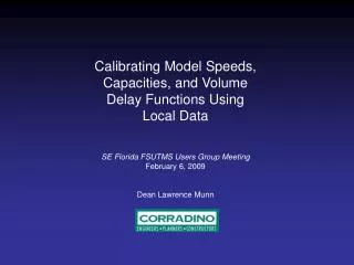
This presentation discusses the calibration of traffic demand models focusing on speeds, capacities, and volume-delay functions using local data in Southeastern Florida. Presented during the FSUTMS Users Group Meeting on February 6, 2009, by Dean Lawrence Munn, it highlights improvements achieved through enhanced model outputs, validation processes, and applications across various projects such as the Indiana Statewide Travel Demand Model, Genesee County Model, and Maricopa Association of Governments Model. It underscores methodologies for speed assumptions and capacity adjustments that enhance modeling accuracy and realism.

Enhancing Traffic Demand Models with Local Data Calibration in Southeastern Florida
E N D
Presentation Transcript
Calibrating Model Speeds, Capacities, and Volume Delay Functions Using Local Data SE Florida FSUTMS Users Group Meeting February 6, 2009 Dean Lawrence Munn
Reasons for Improving • Model outputs are more realistic and detailed • Model validation process and outcome improved • Models are sensitive to more project types • Model applications are easier to defend
Some Recent Projects: • Indiana Statewide Travel Demand Model • Genesee County, Michigan Model • Maricopa Association of Governments Model
Indiana Statewide Travel Demand Model • Current model covers 87,000 sq miles • Model network has 45,000 links, but only covers Minor Collector or higher • TAZ system has 4700 zones • Extends into neighboring states, includes major metro areas • Contains detailed data
Indiana Statewide Travel Demand Model Free-flow Speed Assumptions • Speed assumptions have evolved over time • Use real posted speed from roadway data files • Modify posted speed for advisory speeds (no passing, horiz. curves, etc.) • Modify posted speed using data gathered from actual travel speeds • Combine travel speed and intersection delay into composite travel time
Indiana Statewide Travel Demand Model Free-flow Speed • Developed for I-69 Tier 1 EIS • Incorporated into ISTDM v 4 • Takes estimated posted speeds • Adjusts for actual driver behavior • Data came from 26 county GPS speed survey • This methodology has been implemented in multiple MPO models
Indiana Statewide Travel Demand Model Free-flow Speed Accounting for Intersection Delay • Intersection capability developed for I-69 Tier 1 EIS • Incorporated into ISTDM v 4 • Adjusts travel times to account for signal delays • Method transferred to several MPO models • Recent MPO models have enhanced capabilities
Indiana Statewide Travel Demand Model Development of Model Capacities • Computing an HCM compatible capacity from link attributes • Originally developed for the Indiana Statewide Model • Applied on a link by link basis • Documented in NCHRP 358 as a best practice • Subsequently implemented in many models Variables Used: • Speed • Number of Lanes • Functional Classification • Access Control • Median Type • Lane Width • Shoulder Width • Pct. Heavy Vehicles • Interchange Density • Access Points per Mile
Indiana Statewide Travel Demand Model Calibrating Model Capacities Adjustment to Capacity for Signal Delay • Signal delay is accounted for in capacity instead of VDF • Capacity reduction factor is a ratio of flow rates • Similar effect as VDFs with signal delay • Advantage is simplicity at assignment stage
Indiana Statewide Travel Demand Model Calibrating Volume-Delay Functions • Original work done in 1996-97 at INDOT • INDOT calibrated BPR alphas and betas • INDOT ATR data covered multiple road classes • INDOT had a handful of locations for each class • BPR alpha and beta parameters were developed and coded as link attributes
Genesee County Michigan Model • Current model covers 652 sq miles • Model network has 4300 links • TAZ system has 676 zones • Network contains detailed Michigan Geographic Framework data
Genesee County Michigan Model Free-flow Speed Assumptions More Advanced GPS Survey Applications • Methodology developed for AMBAG model • Used for Genesee Model • Being applied for Phoenix Model
Min Max Tn-1 Tn T1 Correspond Model Link End Time Start Time Model Link TL TL = Max - Min Genesee County Michigan Model Free-flow Speed Assumptions Computing Space-Mean Speed from GPS
Genesee County Michigan Model Free-flow Speed Assumptions Computing Space-Mean Speed from GPS – Separating Signals and Mid-Block • Information is used to adjust mid-block free flow speed from posted speed • Also used to add travel time for intersection delay • Actual GPS data by corridor was used to verify accuracy of Speed-Cap program
Maricopa Association of Governments Model • Started major model update in 2008, activity based model • Current model covers 11,000 sq miles • Model network has 22,000 links, but only covers Minor Arterial or higher • TAZ system has 2000 zones • Dean was PM on supply-part modeling tasks (network) • Project is on-going
Maricopa Association of Governments Model Free-flow Speed Assumptions • Obtain travel speeds from GPS survey covering ¾ of road network • Obtain travel speeds from loop detector data (~40 locations) • Test travel speeds from other ITS detectors (radar, passive acoustic) • Used the same methodology used for Genesee, Michigan • Final product was a new speed lookup table
Maricopa Association of Governments Model Calibrating Model Capacities Using Typical Profiles
Calibrating Model Capacities Using Typical Profiles
Maricopa Association of Governments Model Calibrating Model Capacities The Problem of Multi-Hour Time Periods • HCM only provides guidance for one hour capacities • With uniform temporal distribution, multiply by number of hours • Real traffic is not uniformly distributed over time • Period-specific directional and peak factors have to be developed
Calibrating Volume-Delay Functions • Phoenix project used extensive loop detector data • Phoenix data limited to freeways and a few arterials • Phoenix data allowed some testing of variability by area type
Calibrating Volume-Delay Functions Freeway Loop Detector Data
Calibrating Volume-Delay Functions Freeway Loop Detector Data
Calibrating Volume-Delay Functions Signalized Arterial Loop Detector Data
Calibrating Volume-Delay Functions Curve Parameter Calibration and Evaluation Process
Thank You Any Questions?