Download
1 / 13
130 likes | 270 Views
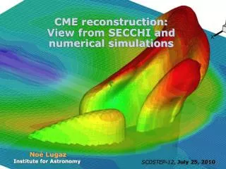
CME reconstruction: View from SECCHI and numerical simulations. Noé Lugaz Institute for Astronomy. SCOSTEP-12 , July 25, 2010. Using MHD Simulations. 3-D MHD Simulation Synthetic Images produced (LOS, EUV, in-situ, etc…)

E N D
CME reconstruction:View from SECCHI and numerical simulations Noé Lugaz Institute for Astronomy SCOSTEP-12, July 25, 2010
Using MHD Simulations 3-D MHD Simulation Synthetic Images produced (LOS, EUV, in-situ, etc…) Analysis technique is applied (mass, energetics, direction, kinematics) Comparison with the simulated “truth” Play with the input (parametric study) Error of the method is quantified
Using MHD Simulations • Best way to quantify the errors intrinsic to the methods. • MHD simulations can be used as constrained tests, by varying the input. CME mass calculated from the 3-D MHD simulation. CME mass calculated from the white-light LOS images. Lugaz et al., ApJ, 627, 2005 • Mass can be derived from single coronagraph images (following Vourlidas et al., 2002) • Mass is about 50% underestimated. • Indirect confirmation by STEREO.
Comparing 3-D structure of CMEs with LOS images • Left: LOS images. • Right: 3-D simulation. • Blue: density decrease over background. • Red: density increase. • Close to the Sun, the core and cavity are still clearly visible. • Farther away, line-of-sight effects make it harder to distinguish low and high-density regions, and to estimate the extent of the CME.
Example for Jan. 24-25, 2007 CMEs • 2 CMEs 16 hours apart. • 2nd CME is about twice faster than 1st CME. • Data gap in SECCHI coverage at the time of the expected interaction. • After data gap: 3 bright fronts. What’s their origin? Running difference of density on the Thomson sphere, running difference HI-2 images Lugaz et al., ApJL., 2008
J-maps (time-elongation plots) Time (from 01/25)-elongation plots for PA 69 (apparent central PA of SECCHI). Procedure developed by Sheeley et al. for LASCO data. Lugaz et al., Sol. Phys, 2009
2- Different PA, different view Time (from 01/25)-elongation plots for PA 90 (approx. nose of CMEs).
Advantages and limitations • Advantages: • Thomson scattered signal calculated from the 3-D distribution of density. • Can separate observational effects from physical characteristics. • No assumption of shape/symmetry. • “Realistic” solar wind. • Limited assumptions: • MHD. • Out-of-equilibrium flux ropes. But in the heliosphere, the exact CME initiation mechanism is of limited importance. • Initial CME magnetic energy is set to reproduceLASCO speed. • Cannot be used for every (Earth-directed) CME. • Other simulations (e.g., ENLIL) can be used for almost every Earth-directed CME but no magnetic field in CME (and initiation at 20 RSun).
Stereoscopic view in HIs • Only a few CMEs have been observed simultaneously in the 2 HIs. • What can we learn about CMEs ?
Analytical model to derive CME radius • Assumptions: • CME front is locally circular. Its radius is unknown and varies with time. • Direction of the CME is constant AND KNOWN. Here, we use the value derived by Thernisien et al. in COR (-21o). • The two STEREO spacecraft observe the front at the elongation angle corresponding to the tangent to this front • Here, ST-A determines the CME nose position, ST-B the CME radius. Asymmetry of measurements can be explained by expansion/ shrinking of the CME due internal pressure and interaction of the CME with solar wind. 2 viewpoints can be used to derive the CME radius. Lugaz et al., ApJ, 2010
Formula and results CME direction elongation separation STA-Earth radius ST-A distance distance We used measurements made by NRL and RAL based on J-maps. Fast changes when the CME is observed in COR2-B and HI1-A. Rate after 20 hours (from 0.25 to 0.65 AU): -4o/day. Forecast at 1 AU: hit at ST-B at 03:00UT on 04/30. No hit at ST-A and ACE. Reality: ICME from 15:30 on 04/29 to 07:00 on 04/30
Other models Thernisien et al., 2009, Sol. Phys Wood & Howard, 2009, ApJ • Angular extent consistent with Thernisien et al., Sol Phys, 2009 (~ 21o) and with Wood & Howard (~ 20o for the outer edge) • Decreasing cross-section appears to be caused by the NE direction of the CME (w/r to ST-B) resulting in the leg of the CME. Almost a “mapping”
Conclusions • MHD simulations can be used to test different analysis methods. • We have the ability to do synthetic line-of-sight images and J-maps from 3-D MHD code and compare with the 3-D structure. • Running difference and J-mapping result in a loss of information. We must be careful. • How to use stereoscopic heliospheric observations? • Simple geometrical model to derive CME expansion, • Visual fitting/Forward modeling. • More work to develop analysis methods and/or more numerical simulations is required to better understand HI measurements. These studies have been made possible by the following grants: NSF-CAREER ATM0639335, NSF-NSWP ATM0819653 and NASA-LWS NNX08AQ16G.