Problem

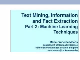
Text Mining, Information and Fact ExtractionPart 2: Machine Learning Techniques Marie-Francine MoensDepartment of Computer ScienceKatholieke Universiteit Leuven, Belgiumsien.moens@cs.kuleuven.be

Problem • Symbolic techniques are useful in very restricted subject domains that exhibit standard patterns: • e.g., mining of a weather report • In most settings language is characterized by: • a variety of patterns that express the same or similar meanings • ambiguous patterns that receive their meaning based on the context • Patterns change in time (e.g., blog and chat languages) © 2008 M.-F. Moens K.U.Leuven

Problem • manual effort is huge to build all the needed (contextual) patterns for all kinds of information extraction tasks • IE in terrorism domain: experiment of Riloff (1996): automatic construction of dictionary of extraction patterns from an annotated training corpus achieved 98% of the performance of handcrafted patterns => machine learning of extraction patterns [Riloff AI 1996] © 2008 M.-F. Moens K.U.Leuven

Problem • Since 1996: interest in machine learning for information extraction: • Usually supervised learning algorithms: • e.g., learning of rules and trees, support vector machines, maximum entropy classification, hidden Markov models, conditional random fields • Unsupervised learning algorithms: • e.g., clustering (e.g., noun phrase coreferent resolution) • Weakly supervised learning algorithms © 2008 M.-F. Moens K.U.Leuven

Overview • Features • Supervised methods: • Support vector machines and kernel methods • Probabilistic models: • Naive Bayes models • Maximum entropy models (exemplary results are added) © 2008 M.-F. Moens K.U.Leuven

Generative versus discriminative classification • In classification: given inputs x and their labels y: • Generative classifier learns a model of the joint probabilityp(x,y)and makes its predictions by using Bayes’ rule to calculatep(y|x) and then selects the most likely labely: • e.g.,Naive Bayes, hidden Markov model • to make computations tractable: simplifying independence assumptions © 2008 M.-F. Moens K.U.Leuven

Generative versus discriminative classification • Discriminative classifier is trained to model the conditional probability p(y|x) directly and selects the most likely labely, or learns a direct map from inputs x to the class labels: • e.g.,maximum entropy model, support vector machine • better suited when including rich, overlapping features © 2008 M.-F. Moens K.U.Leuven

Maximum entropy principle • Text classifiers are often trained with incomplete information • Probabilistic classification can adhere to the principle of maximum entropy: When we make inferences based on incomplete information, we should draw them from that probability distribution that has the maximum entropy permitted by the information we have: e.g., • maximum entropy model, conditional random fields © 2008 M.-F. Moens K.U.Leuven

Combining classifiers • Multiple classifiers are learned and combined: • Bagging: e.g., sample of size n is taken randomly with replacement from the original set of n trainingdocuments • Adaptive resampling: no random sampling, but objective = to increase the odds of sampling documents that previously induced classifiers have erroneously been classified • Stacking: predictions from different classifiers are used as input for a meta-learner • Boosting: generating a sequence of classifiers, after each classification greater weights are assigned to objects with an uncertain classification, and classifier is retrained © 2008 M.-F. Moens K.U.Leuven

Feature selection and extraction • In classification tasks: object is described with set of attributes or features • Typical features in text classification tasks: • word, phrase, syntactic class of a word, text position, the length of a sentence, the relationship between two sentences, an n-gram, a document (term classification), …. • choice of the features is application- and domain-specific • Features can have a value, for text the value is often: • numeric, e.g., discrete or real values • nominal, e.g. certain strings • ordinal, e.g., the values 0= small number, 1 = medium number, 2 = large number © 2008 M.-F. Moens K.U.Leuven

Feature selection and extraction • The features together span a multi-variate space called the measurement space or feature space: • an objectxcan be represented as: • a vector of features: x = x1, x2, …, xpT where p = the number of features measured • as a structure: e.g., • representation in first order predicate logic • graph representation (e.g., tree) where relations between features are figured as edges between nodes and nodes can contain attributes of features © 2008 M.-F. Moens K.U.Leuven

Feature selection • = eliminating low quality features: • redundant features • noisy features • decreases computational complexity • decreases the danger of overfitting in supervised learning (especially when large number of features and few training examples) • increases the chances of detecting valuable patterns in unsupervised learning and weakly supervised learning • Overfitting: • the classifier perfectly fits the training data, but fails to generalize sufficiently from the training data to correctly classify the new case © 2008 M.-F. Moens K.U.Leuven

Feature selection • In supervised learning: • feature selection often incorporated in training algorithms: • incrementally add features, discard features, or both, evaluating the subset of features that would be produced by each change (e.g., algorithms that induce decision trees or rules from the sample data) • feature selection can be done after classification of new objects: • by measuring the error rate of the classification • those features are removed from or added to the feature set when this results in a lower error rate on the test set © 2008 M.-F. Moens K.U.Leuven

Feature extraction • = creates new features by applying a set of operators upon the current features: • a single feature can be replaced by a new feature (e.g., replacing words by their stem) • a set of features is replaced by one feature or another set of features • use of logical operators (e.g., disjunction), arithmetical operators (e.g., mean, dimensionality reduction) • choice of operators: application- and domain-specific • In supervised learning can be part of training or done after classification of new objects © 2008 M.-F. Moens K.U.Leuven

Support vector machine (SVM) • Discriminant analysis: • determining a function that in a best way discriminates between two classes • text categorization: two classes: positive and negative examples of a class • e.g.,linear discriminant analysisfinds a linear combination of the features (variables) : hyperplane (line in two dimensions, plane in three dimensions, etc.) in the p-dimensional feature space that best separates the classes • usually, there exist different hyperplanes that separate the examples of the training set in positive and negative ones © 2008 M.-F. Moens K.U.Leuven

Support vector machine • Support vector machine: • when two classes are linearly separable: • find a hyperplane in the p-dimensional feature space that best separates with maximum margins the positive and negative examples • maximum margins: with maximum Euclidean distance (= margin d) to the closest training examples (support vectors) • e.g., decision surface in two dimensions • idea can be generalized to examples that are not necessarily linearly separable and to examples that cannot be represented by linear decision surfaces © 2008 M.-F. Moens K.U.Leuven

Support vector machine • Linear support vector machine: • case: trained on data that are separable (simple case) • input is a set of ntraining examples: where xi and yi  {-1,+1} indicating that xiis a negative or positive example respectively © 2008 M.-F. Moens K.U.Leuven

Support vector machine Suppose we have some hyperplane which separates the positive from the negative examples, the points which lie on the hyperplane satisfy: where w = normal to the hyperplane = perpendicular distance from the hyperplane to the origin = Euclidean norm of w © 2008 M.-F. Moens K.U.Leuven

let d+(d-) be the shortest distance from the separating hyperplane to the closest positive (negative) example define the margin of the separating hyperplane to be d+ and d- search the hyperplane with largest margin Given separable training data that satisfy the following constraints: for yi =+1 (1) for yi = -1 (2) which can be combined in 1 set of inequalities: for i = 1,…, n (3) © 2008 M.-F. Moens K.U.Leuven

The hyperplane that defines one margin is defined by: with normal w and perpendicular distance from the origin The hyperplane that defines the other margin is defined by: with normal w and perpendicular distance from the origin Hence d+ = d- = and the margin= © 2008 M.-F. Moens K.U.Leuven

Hence we assume the following objective function to maximize the margin: A dual representation is obtained by introducing Lagrange multipliers i, which turns out to be easier to solve: (4) © 2008 M.-F. Moens K.U.Leuven

Yielding the following decision function: (5) The decision function only depends on support vectors, i.e., for which i > 0. Training examples that are not support vectorshave no influence on the decision function © 2008 M.-F. Moens K.U.Leuven

Support vector machine • Trained on data not necessarily linearly separable (soft margin SVM): • the amount of training error is measured using slack variables ithe sum of which must not exceed some upper bound • The hyperplanes that define the margins are now defined as: • Hence we assume the following objective function to maximize the margin: © 2008 M.-F. Moens K.U.Leuven

Support vector machine • When classifying natural language data, it is not always possible to linearly separate the data: in this case we can map them into a feature space where they are linearly separable • Working in a high dimensional feature space gives computational problems, as one has to work with very large vectors • In the dual representation the data appear only inside inner products (both in the training algorithm shown by (4) and in the decision function of (5)): in both cases a kernel function can be used in the computations © 2008 M.-F. Moens K.U.Leuven

Kernel function • A kernel function K is a mapping K: S x S0,  from the instance space of training examples S to a similarity score: • In other words a kernel function is an inner product in some feature space • The kernel function must be: • symmetric K(xi,xj) = K(xj,xi) • positive semi-definite: if x1,…,xnS, then the n x n matrix G (Gram matrix or kernel matrix)defined by Gij= K (xi,xj) is positive semi-definite* * has non-negative eigenvalues © 2008 M.-F. Moens K.U.Leuven

Support vector machine • Advantages: • SVM can cope with many (noisy) features: no need for a priori feature selection, though you might select features for reasons of efficiency • many text categorization problems are linearly separable © 2008 M.-F. Moens K.U.Leuven

Kernel functions • Typical kernel functions: linear (mostly used in text categorization), polynomial, radial basis function (RBF) • In natural language: data are often structured by the modeling of relations=> kernels that (efficiently) compare structured data: e.g., • Rational kernels = similarity measures over sets of sequences • n-gram kernels • convolution kernels • Kernels on trees © 2008 M.-F. Moens K.U.Leuven

n-gram kernels • n-gram is a block of adjacent characters from an alphabet  • n-gram kernel: to compare sequences by means of subsequences they contain: #(sxi) #(sxj) where #(sx) denotes the number of occurrences of s in x • the kernel function can be computed in O(xi + xj) time and memory by means of a special suited data structure allowing one to find a compact representation of all subsequences in xin onlyO(x) time and space [Vishwanathan & Smola 2004] © 2008 M.-F. Moens K.U.Leuven

Convolution kernels • Object x X consists of substructures xp Xp where 1pr and r denotes the number of overall substructures • Given the set of all possible substructures P(X), one can define a relation R (e.g., part of) between a subset of P and the composite object x • Given a finite number of subsets, R is called finite • Given a finite relation R,R-1 defines the set of all possible decompositions ofxinto its substructures: R-1(x)= {z P(X): R (z, x)} © 2008 M.-F. Moens K.U.Leuven

Convolution kernels • The R-convolutionkernel: is a valid kernel with Kibeing a positive semi-definite kernel on Xi • The idea of decomposing a structured object into parts can be applied recursively so that one only requires to construct kernels over the “atomic” parts of Xi © 2008 M.-F. Moens K.U.Leuven

Tree kernels • Based on convolution kernels • A tree is mapped into its sets of subtrees, the kernel between two trees K(xi, xj) is then computed by taking the weighted sum of all terms between both trees • Efficient algorithms to compute the subtrees: • O(xi.xj), where x is the number of nodes of the tree • O(xi+xj), when restricting the sum to all proper rooted subtrees [Collins & Duffy 2004] [Vishwanathan & Smola 2004] © 2008 M.-F. Moens K.U.Leuven

Tree kernels • Comparison of augmented dependency trees for relation extraction from sentences: • recursive function to combine parse tree similarity with similarity s(xi, xj) based on feature correspondence of the nodes of the trees where m(xi, xj)  {0, 1} determines whether two nodes are matchable or not c = children subtrees © 2008 M.-F. Moens K.U.Leuven

Naive Bayes (NB) model • Bayesian classifier: • the posterior probability that a new, previously unseen object belongs to a certain class given the features of the object is computed: • based on the probabilities that these individual features are related to the class • NaiveBayes classifier: • computations simplified by the assumption that the features are conditionally independent © 2008 M.-F. Moens K.U.Leuven

Naive Bayes model • Estimations from training set: • P(Cj) • P(wi|Cj): • binomial or Bernoulli model: • fraction of objects of class Cj in which feature wi occurs • multinomial model: • fraction of times that feature wi occurs across all objects of class Cj • additional positional independence assumptions • To avoid zero probabilities: add one to each count (add-one or Laplace smoothing) © 2008 M.-F. Moens K.U.Leuven

Naive Bayes model • Class assignment: • find the k most probable classes; k = 1: • alternative: select classes for which • Advantages: • Efficiency • Disadvantages: • Independence assumptions • No accurate probability estimates: close to 0; winning class after normalization close to 1 © 2008 M.-F. Moens K.U.Leuven

Maximum entropy principle • Used in classifiers that compute a probabilistic class assignment • Maximum entropy principle: given a set of training data, model what is known and assume no further knowledge about the unknowns by assigning them equal probability • In other words we choose the model p* that preserves as much uncertainty as possible between all the models p  Pthat satisfy the constraints enforced by the training examples • Examples: • maximum entropy model • conditional random field © 2008 M.-F. Moens K.U.Leuven

Maximum entropy model • Given n training examples S = {(x, y)1,…,(x, y)n}. where x = feature vector and y = class • We choose the model p* that preserves as much uncertainty as possible, or which maximizes the entropy H(p) between all the models pP that satisfy the constraints enforced by the training examples: H(p) = © 2008 M.-F. Moens K.U.Leuven

Problem

Problem

Presentation Transcript

PROBLEM SOLVING PROBLEM POSING

Problem

Problem

Problem

Problem

Problem

PROBLEM

Problem:

Problem

problem

Problem

Problem

Problem

Chapter 6 Problem 3 Problem 5 Problem 6 Problem 12

Problem