Download
1 / 26
260 likes | 355 Views
Explore rainfall estimation using Areal R(ΦDP) and R(KDP) by BMRC C-Pol radar. Analyze radar-raingauge comparisons in varied area sizes. Correct wind drift effects for accurate results. Learn about optimal offset vector analysis and correcting wind drift. Consider DSD variability for accurate rain rate estimates.

E N D
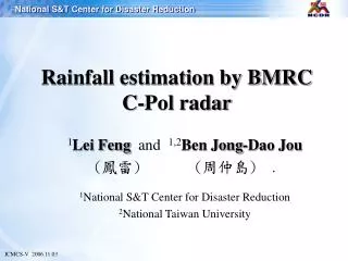
Rainfall estimation by BMRC C-Pol radar 1Lei Feng and 1,2Ben Jong-Dao Jou (鳳雷) (周仲島). 1National S&T Center for Disaster Reduction 2National Taiwan University ICMCS-V2006.11.03
To illustrate the ability of rainfall estimation using Areal R(ΦDP) and R(KDP) by BMRC C-Pol radar. Radar-Raingauge comparisons in three different sizes of area : Multi-beam (Area ~100 km2) Areal R(ΦDP) Single-beam (Area ~ 25 km2) Areal R(ΦDP) Point (Area ~ 2 km2) R(KDP) Try to correct the wind drift effect when comparing with single raingauge. Objectives
NSSL Ryzhkov and Zrnic(1998) CSU Bringi (2001) 1 Two Areal Rainfall schemes Notice the difference: Gate area ↑ with range ↑ but NSSL scheme without area weighting Keep the area weighting, but need ΦDP information at each range gate
BMRC C-Pol rain gaugenetwork 5 single-beams, the area of each beam is ~ 25 km2 1 multi-beam, the area of each beam is ~ 100 km2 18 raingauges, the radar coverage of each gauge is ~ 2 km2 (radius 0.8 km) RD-69 In Darwin 18 rain gauges in the 10 x 10 km2 area C-Pol radar at (0,0)
Case A - 15 Jan 1999 Case A, Time series plot (100 km2)
Case B - 01 Mar 1999 Case B, Time series plot (100 km2)
Case C - 17 Mar 1999 Case C, Time series plot (100 km2)
Area size: ~100 km2 Very high correlation coefficient: 0.97 Small standard deviation: 1.99 mm/hr Little underestimate Sample number: 108 Multi-beam results case (A+B+C)
Area size: ~25 km2 High correlation coefficient: 0.94 Small standard deviation: 3.43mm/hr Little underestimate Sample number: 590 Single-beam results case (A+B+C)
Area size: ~2 km2 Low correlation coefficient: 0.86 Large standard deviation: 6.38mm/hr Under estimation Sample number: 1091 Point results case (A+B+C) • The result is getting worse as the verification area getting smaller. Why ?
Zawadzki (1975) already described Radar-Gauge comparison problems: Wind drift effect Time lag effect Point Comparison Problems • Inherence difference of the measurements: Rain gauge accumulates continuously rainfall on a point while radar samples almost instantaneously a volume averaged rainfall rate.
Can we correct the wind drift effect ? Strong horizontal wind Overestimate or Underestimate ? from DLOC How about the wind drift effect ?
An area of radar data which covering all surface rain gauges is moved around the original point in a square window (8km x 8km) with 200 m interval in X and Y direction. The cross-correlation coefficient is calculated between the time lagged (1.5 minute) surface rain rates of the gauges and the space shifted radar rain rates. A two-dimensional correlation field is produced. The distance from the point of the maximum correlation to the original point was defined as “optimal offset” of the horizontal displacement. Optimaloffsetvector
Is these two reasonable ? Case C Case A Case B 2 km Only 39/89 volumes can be easily found out the offset vectors, most of them are convective type rain.
Checking the optimal vector far from system moving velocity case
No wind drift correction After wind drift correction Case B Case A
after wind drift correctionBut significant underestimation No wind drift correction If the coefficient of R(KDP) estimator increase 50%, it look better. Can we do this change for this case ?
Rainfall with smaller raindrops need to use higher coefficient in R(KDP) estimator small Zdr ~ small Do big Zdr ~ big Do Adopted from L. D. Carey ATMO 689
Volume median diameter D0 estimation Disdrometer observation Radar estimation Note: the comparison here is not the same case, but are similar squall line type precipitation in Darwin.
No wind drift correction After wind drift correction
It’s very important to consider the wind drift effect when doing single point radar-gauge comparison. In this study, the normalized error has 17% improvement. summary (1) Correlation Coefficient of radar-raingauge comparison
summary (2) • Use the BMRC C-Pol radar phase base estimator to estimate rain rate is very accurate , especially on convective rainfall. • For accurate rain rate estimation, it needs to consider the DSD variability such as stratiform rainfall, orographic rainfall, shallow convective warm rain and so on when using R(KDP) estimator. Thanks !
Optimal vector Finding, 06:40 15-Jan-1999 (C-Pol at Darwin) Lag 0 min Lag 1 min Lag 2 min Lag 3 min Lag 4 min Lag 5 min