Download
1 / 26
260 likes | 283 Views
Explore practical uses of terrain conductivity measurements in dissecting subsurface geological problems. Learn how to constrain geophysical problems and develop subsurface models with examples.

E N D
Subsurface model development using terrain conductivity measurements The problems in the text provide insights into the practical uses of terrain conductivity measurements to dissect subsurface geological problems. In all the text examples the geologist and geophysicist have information about some of the variables so they can answer a specific question about the subsurface. Information used to constrain geophysical problems can come from outcrop, auger and borehole measurements. Tom Wilson, Department of Geology and Geography
Problem 8.5 In problem 8.5, the geologist/geophysicist have information that helps constrain the problem to that of determining 2. In this case a can be interpreted in terms of 2 since the thickness of the surface layer is known. When you add the air layer you have a 2z, 3 layer problem. Tom Wilson, Department of Geology and Geography
Problem 8.6 In this problem the geologist & geophysicist know there are gravel deposits scattered through the glacial till. The gravel deposits serve to localize fresh water accumulations that could be used as a domestic water supply. Auger holes, for example, could provide information about d1 and the three s so that thickness can be estimated. 1st 2nd layer is the gravel 3rd Tom Wilson, Department of Geology and Geography
Problem 8.7 In this problem, the geologist knows the near surface geology consists of a soil layer with known conductivity (30mS/m) covering granitic bedrock of known conductivity (0.1mS/m). This allows variations in apparent conductivity to be translated into a bedrock depth profile or map. Tom Wilson, Department of Geology and Geography
Developing a subsurface model – some examples: buried druim Tom Wilson, Department of Geology and Geography
Modeling igneous intrusion with gravity and magnetic data Tom Wilson, Department of Geology and Geography
Complex normal faulted structure with syndepositional variations in sediment thickness (grav and mag) Tom Wilson, Department of Geology and Geography
Questions about 8.5, 8.6, 8.7? Organize your presentation! • What are you solving for? • List given variables associated with the problem • Show calculations for additional variables needed to solve the problem. • Show calculations used to calculate requested quantity • Highlight your results (draw a box around answers sought in the problem). Some of you are still having difficulty organizing your work. Put some additional effort into preparing your work. Tom Wilson, Department of Geology and Geography
On your list … Today – introductory terrain conductivity modeling with IX1D Chapter 8 problems due this Thursday (Sept. 3)Problems 8.5, 8.6 & 8.7 Begin reading the resistivity chapter (Chapter 5) in Berger, Sheehan and Jones Writing section should get the chapter summary outline in next Tuesday, September 8th. The terrain conductivity paper summary will be due on Thursday September 10th. Tom Wilson, Department of Geology and Geography
Next we’ll get into the Terrain Conductivity/Resistivity Modeling Software IX1D A full set of terrain conductivity measurements obtained from the EM31 and EM34 provides 8 values of apparent conductivity. The variations of apparent conductivity can be used to answer more complicated questions about subsurface geology. However, considerable geological and geophysical information is required to help constrain the solutions or subsurface models that explain apparent conductivity variations. Tom Wilson, Department of Geology and Geography
First – go to the common drive and copy over the file folder Tom Wilson, Department of Geology and Geography
From your programs list > find IX1Dv2 Drop into this folder, Right click and drag the icon to your desktop. When you lift up, select create shortcut Tom Wilson, Department of Geology and Geography
First - locate and bring up IX1D IX1D Software should come up with no problem. You may have to run the program by going directly to the programs folder on your C:\Drive Change the default name to Your name. I think it requires 12 characters, so you could add G454 If needed – Enter Access Code 307609922 Tom Wilson, Department of Geology and Geography
You’ll get a plot that will look something like this. Don’t worry about that right now. We just want to be sure the software comes up. Two plots: data on left and model on right Tom Wilson, Department of Geology and Geography
Recall that using both the EM31 and EM34 in combination we can collect 8 data points Computer gets about 18, while our hand computations gave us about 20 mS/m The 4 horizontal dipole apparent conductivity measurements are shown using purple squares Horizontal Vertical log scale The 4 vertical dipole apparent conductivity measurements are shown using purple squares Quasi - Depth Effective Penetration Depths Think of this as depth beneath the surface log scale Tom Wilson, Department of Geology and Geography
The Terrain Conductivity Lab Exercise is designed around the use of data obtained using the EM31 and EM34 terrain conductivity meters Find & open EM1.IXR Data set EM1.IXR is in folder IX1D-TC Typical survey yields 8 measurements consisting of one set of measurements made with the vertical dipole orientation and one set with horizontal dipole orientation Tom Wilson, Department of Geology and Geography
IX1D Display window – basic tour >The data are in the IX1D-TC folder Subsurface conductivity model Open the EM1 data set 50mS/m Horizontal Dipole measurements 10mS/m Vertical Dipole measurements 15mS/m Tom Wilson, Department of Geology and Geography
Vertical Dipole measurements ~12.6m ~51m ~4.7m ~25.5m Effective Penetration Depths (keep their limited significance in mind) 5.5m 15m 30m 60m Tom Wilson, Department of Geology and Geography
Remember the skin depth is the depth at which the signal strength drops to 1/e of its source amplitude. http://www.geo.wvu.edu/~wilson/emvrz.xls REMEMBER- Although the area under the curve beneath 4.7 meters equals 37% of the total area, intervals beneath that depth can be responsible for more than 37% of the measured apparent conductivity! Tom Wilson, Department of Geology and Geography
Vertical Dipole measurements ~12.6m ~51m ~4.7m ~25.5m “Effective Penetration Depths” correspond to depths at which remaining area on the relative response function is ~37% of the total area. 5.5m 15m 30m 60m 3.67m 10m 20m 40m Tom Wilson, Department of Geology and Geography
At this point, make sure you have IX1D open There should be no problems but … If some of you are unable to get the program up and running, double up – share a computer. I’ll note computers and try to get everything up and running before this Thursday. Tom Wilson, Department of Geology and Geography
Did everyone get the IX1D-TC folder copied to their network (N:) drive? Then Bring up IX1D v2 from the start programs window or … Do a file> open and navigate to your N:\Drive IX1D-TC and open the file EM1. Note that EM1 –EM6 are for practice and EM7 through 12 are for the lab. The data display may come up showing resistivity instead of conductivity Tom Wilson, Department of Geology and Geography
Developing a subsurface cross section from your terrain conductivity models Tom Wilson, Department of Geology and Geography
Let’s work through some of these soundings.Refer to your handout. All steps and more are illustrated in today’s “Exploring IX1D …” handout. Do a file> open and navigate to your G:\Drive IX1D-TC and open the file EM1. Note that EM1 –EM6 are for practice and EM7 through 12 are for the lab. Tom Wilson, Department of Geology and Geography
Pick a sounding (EM2-6), determine the conductivity and thickness of the contaminated zone and Turn in before leaving See page 15 of today’s handout Fill in the blanks, tear off and submit before leaving. I’ll spend some time outside the slides showing you how to develop your model. Tom Wilson, Department of Geology and Geography
Next Week Today – introductory terrain conductivity modeling with IX1D Chapter 8 problems due this Thursday (Sept. 3)Problems 8.5, 8.6 & 8.7 Begin reading the resistivity chapter (Chapter 5) in Berger, Sheehan and Jones Writing section should get the chapter summary outline in ______________. Tom Wilson, Department of Geology and Geography