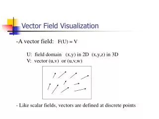
Vector Field Visualization
Vector Field Visualization. Jian Huang, CS 594, Spring 2002 This set of slides reference slides developed by Prof. Torsten Moeller, at CS, Simon Fraser Univ., BC, Canada. Vector Visualization. Data set is given by a vector component and its magnitude

Vector Field Visualization
E N D
Presentation Transcript
Vector Field Visualization Jian Huang, CS 594, Spring 2002 This set of slides reference slides developed by Prof. Torsten Moeller, at CS, Simon Fraser Univ., BC, Canada
Vector Visualization • Data set is given by a vector component and its magnitude • often results from study of fluid flow or by looking at derivatives (rate of change) of some quantity • trying to find out what to see and how! • Many visualization techniques proposed
Vector Visualization - Techniques • Hedgehogs/glyphs • Particle tracing • stream-, streak-, time- & path-lines • stream-ribbon, stream-surfaces, stream-polygons, stream-tube • hyper-streamlines • Line Integral Convolution
Vector Visualization - Origin • Where are those methods coming from?? • Rich field of Fluid Flow Visualization • Hundreds of years old!! • Modern domain - Computational Field Simulations
Flow Visualization • Gaseous flow: • development of cars, aircraft, spacecraft • design of machines - turbines, combustion engines • Liquid Flow: • naval applications - ship design • civil engineering - harbor design, coastal protection • Chemistry - fluid flow in reactor tanks • Medicine - blood vessels, SPECT, fMRI
Flow Visualization (2) • What is the problem definition? • Given (typically): • physical position (vector) • pressure (scalar), • density (scalar), • velocity (vector), • entropy (scalar) • steady flow - vector field stays constant • unsteady - vector field changes with time
Vector Visualization - Goal • What are we looking for? • Very good question! Some understanding! ANY UNDERSTANDING!
Flow Visualization - traditionally • Traditionally - Experimental Flow Vis • How? - Three basic techniques: • adding foreign material • optical techniques • adding heat and energy
Experimental Flow Visualiz. • Problems: • the flow is affected by experimental technique • not all phenomena can be visualized • expensive (wind tunnels, small scale models) • time consuming • That’s where computer graphics and YOU come in!
Vector Field Visualization Techniques Local technique:Advection based methods - Display the trajectory starting from a particular location - streamxxxx - contours Global technique: Hedgehogs, Line Integral Convolution, Texture Splats etc. Display the flow direction everywhere in the field
Local technique - Streamline • Basic idea: visualizing the flow directions by releasing particles and calculating a series of particle positions based on the vector field -- streamline
Numerical Integration • Euler • not good enough, need to resort to higherorder methods
Numerical Integration • 2nd order Runge-Kutta
Numerical Integration • 4th order Runge-Kutta
Streamlines (cont’d) - Displaying streamlines is a local technique because you can only visualize the flow directions initiated from one or a few particles - When the number of streamlines is increased, the scene becomes cluttered - You need to know where to drop the particle seeds - Streamline computation is expensive
T=3 T=4 T=2 T=5 timeline T = 2 T = 1 T = 3 Pathlines, Timelines • Extension of streamlines for time-varying data (unsteady flows) • Pathlines: • Timelines: T=1
b.t. =1 b.t. =2 b.t. =3 b.t. =4 b.t. =5 Streaklines • For unsteady flows also • Continuously injecting a new particle at each time step, • advecting all the existing particles and connect them • together into a streakline
Stream-ribbon • We really would like to see vorticities, I.e. places were the flow twists. • A point primitive or an icon can hardly convey this • idea: trace neighboring particles and connect them with polygons • shade those polygons appropriately and one will detect twists
Stream-ribbon • Problem - when flow diverges • Solution: Just trace one streamline and a constant size vector with it:
Stream-tube • Generate a stream-line and connect circular crossflow sections along the stream-line
Stream-balls • Another way to get around diverging stream-lines • simply put implicit surface primitives at particle traces - at places where they are close they’ll merge elegantly ...
Flow Volumes • Instead of tracing a line - trace a small polyhedra
Contours • Contour lines can measure certain quantities by connecting same values along a line
Global techniques - Display the entire flow field in a single picture - Minimum user intervention - Example: Hedgehogs (global arrow plots)
Mappings - Hedgehogs, Glyphs • Put “icons” at certain places in the flow • e.g. arrows - represent direction & magnitude • other primitives are possible
Mappings - Hedgehogs, Glyphs • analogous to tufts or vanes from experimental flow visualization • clutter the image real quick • maybe ok for 2D • not very informative
Global Methods • Spot Noise (van Wijk 91) • Line Integral Convolution (Cabral 93) • Texture Splats (Crawfis 93)
Spot Noise • Uses small motion blurred particles to visualize flows on stream surfaces • Particles represented as ellipses with their long axes oriented along the direction of the flow • I.e. we multiply our kernel h with an amplitude and add a phase shift! • Hence - we convolve a spot kernel in spatial domain with a random sequence (white noise)
Spot Noise • examples of white noise: • set of random values on a grid • Poisson point process - a set of randomly scaled delta functions randomly placed (dart throwing) • variation of the data visualization can be realized via variation of the spot: d - data value m - parameter mapping
Rendering - Spot Noise Different size Different profiles
Rendering - Spot Noise • bla
Rendering - Spot Noise scalar gradients • Scalar - use +-shape for positive values, x-shape for negative values • change the size of the spot according to the norm of the gradient • vector data - use an ellipse shaped spot in the direction of the flow ... flow Velocity potential
Rendering - LIC • Similar to spot noise • embed a noise texture under the vector field • difference - integrates along a streamline LIC Spot Noise
Texture Splats • Crawfis, Max 1993 • extended splatting to visualize vector fields • used simple idea of “textured vectors” for visualization of vector fields
Texture Splats - Vector Viz • The splat would be a Gaussian type texture • how about setting this to an arbitrary image? • How about setting this to an image including some elongated particles representing the flow in the field? • Texture must represent whether we are looking at the vector head on or sideways
Texture Splats Texture images Appropriate opacities
Texture Splats - Vector Viz • How do you get them to “move”? • Just cycle over a periodic number of different textures (rows)
More global techniques Texture Splats