Visualization and Model Intercomparisons of the Vector Vorticity Model

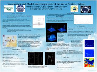
1. Visualization and Model Intercomparisons of the Vector Vorticity Model Nicholas Geyer1, Celal Konor1,Thomas Cram1 Colorado State University, Fort Collins, CO. • Vector Vorticity Model • A three-dimensional anelastic cloud model based on the vorticity equation • The anelastic set of equations maintain a good approximation for cloud dynamics and with the coupling of the vorticity equation allows data to be more straightforward. • This is the first three dimensional model of its kind, as far as we know. • Utilizing vorticity simplifies the problem of boundary conditions at the surface of complex terrains. • Key nonlinear dynamical processes can be more directly implemented and thus lowers the computational requirements. • Prognostic variables: horizontal components of vorticity, potential temperature, mixing ratios of various water phases, and the vertical component of vorticity at the model top. • Previous Tests • Bubble-type test which simulates a warm plume of air • GATE Phase-III: A test of simulating ensemble clouds with full model physics in a large domain. • Model Results • The model produced results beginning at 36 hours after the simulation. This initial 36 hours is regarded as the VVM’s spin up time and all data within the spin-up time may be disregarded. Precipitation • The initial 10 minute run ran from hours 36 to 144 which results in a 6 day run of the entire timeframe. • To continue our analysis, we focused on the greatest maximums and lowest minimums of mean precipitation as shown in FIG 10. FIG 10. Mean precipitation over the entire domain in mm/day • 3-D Visualization • Perhaps one of the most important items to submit to the intercomparison was a 3-D output of what clouds look like after the model simulation at 10 minute intervals. • Utilizing IDL, contour plots of cloud water mass mixing ratio were used to simulate the shapes and locations of clouds over the entire domain. (FIG 5, 6, & 7) • The contour blobs created are stringy and thus may not completely represent a true cloud so further analysis must take place. • In addition, a time lapse animation of our 10 minute output was created to see how the clouds were progressing and advected over the domain • during entire run time. FIG 1. Vertical grid used for discretization FIG 5 (top left), 6 (top right), & 7 (left). Three Dimensional contour plots of Cloud Water mass mixing ratio. There are 100 contoured values from .4 – 1.4 g/kg. The hours shown are 100 (top left), 120 (top right), and 138 (left). Tropical Warm Pool – International Cloud Experiment • This was an experiment that took place in and around Darwin, Australia, from January 20 trhough February 13, 2006. • Noted as the first field program in the tropics that attempted to describe the evolution of tropical convection. • The real measurements were taken by the US Department of Energy’s Atmospheric Radiation Measurement Program, also known as ARM, and a polarmetric weather radar operated by the Australian Bureau of Meteorology. • The purpose of taking the TWP-ICE data was to improve the climate forecasting skills of general circulation models. FIG 8 (right) & 9 (right middle). Cloud Water mass mixing ratio (top) and Vertical velocity (bottom) as measured from Z= 6 km at 138 hours Mixing Ratios and Vertical Velocity • Utilizing both X-Y slices of vertical velocity and cloud water mass mixing ratio, one can infer the location of updraftswith warm most air. • This is like a proxy for cloud locations. The evidence desplayed in FIG 8 & 9 suggests the location of clouds in FIG 7 do make sense. FIG 11 (right bottom). An example of cloud top temperatures in X-Y domain at hour 138. Warmer colors indicate colder clouds. FIG 2. The Domain of the TWP-ICE experiment with locations of measurement apparatuses (Courtesy of ShaochengXie, LLNL) TWP-ICE Model Set-Up Cloud Top Temperatures • In order to reproduce results with the VVM we had to set the model up in exactly the following manner: • Model runs of 16 days (January 18- February 3, 2006) • Horizontal domain size = 176 km X 176 km • Vertical domain size must be greater than 24 km • Periodic boundary conditions • Sea surface temperature must be 29 C with an albedo of .07 • Fully interactive fluxes • Idealized ozone and aerosol profiles from measured observations • Domain-mean large scale forcings are derived from observations • Apply the forcings at full strength below 15 km and zero above 15 km • Nudge obserations every 6 hours • In another effort to identify the location of clouds in the entire domain, we utilized a calculation that found an approximate location of cloud tops via their temperatures according to the cloud water mass mixing ratio and cloud ice mixing ratio. • This better represented the size and coverage of the clouds. Future Work • Continue work with the VVM over new land based and land/ocean cases. • Currently the next test for the VVM is in its planning stages and is the ARM July 1997 study based over Oklahoma, USA. References Fridlind, A. et al., 2009. ARM/GCSS/SPARC TWP-ICE CRM Intercomparison Study. Jung, J., Arakawa, A. 2005. A Three-Dimensional Cloud Model Based on the Vector Vorticity Equation. Atmospheric Science Paper No. 762 Jung, J., 2007. VVCM Technical Report. Ver 1.1. http://kiwi.atmos.colostate.edu/pubs/joon-hee-tech_report.pdf FIG 3 (left) : Ozone sounding profiles for the TWP-ICE domain FIG 4 (right) : Aerosol profile for the TWP-ICE domain