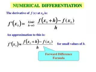
Numerical Differentiation and Integration
Numerical Differentiation and Integration. Standing in the heart of calculus are the mathematical concepts of differentiation and integration :. Figure PT6.1. Figure PT6.2. Noncomputer Methods for Differentiation and Integration.

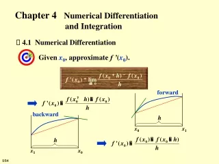
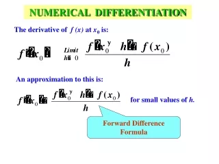
Numerical Differentiation and Integration
E N D
Presentation Transcript
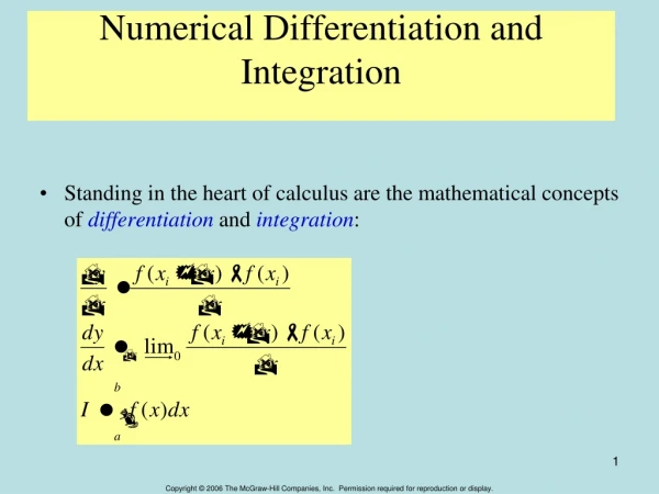
Numerical Differentiation and Integration • Standing in the heart of calculus are the mathematical concepts of differentiation and integration:
Figure PT6.1 Chapter 21
Figure PT6.2 Chapter 21
Noncomputer Methods for Differentiation and Integration • The function to be differentiated or integrated will typically be in one of the following three forms: • A simple continuous function such as polynomial, an exponential, or a trigonometric function. • A complicated continuous function that is difficult or impossible to differentiate or integrate directly. • A tabulated function where values of x and f(x) are given at a number of discrete points, as is often the case with experimental or field data. Chapter 21
Figure PT6.4 Chapter 21
Figure PT6.7 Chapter 21
Newton-Cotes Integration FormulasChapter 21 • The Newton-Cotes formulas are the most common numerical integration schemes. • They are based on the strategy of replacing a complicated function or tabulated data with an approximating function that is easy to integrate: Chapter 21
Figure 21.1 Chapter 21
Figure 21.2 Chapter 21
The Trapezoidal Rule • The Trapezoidal rule is the first of the Newton-Cotes closed integration formulas, corresponding to the case where the polynomial is first order: • The area under this first order polynomial is an estimate of the integral of f(x) between the limits of a and b: Trapezoidal rule
Figure 21.4 Chapter 21
Error of the Trapezoidal Rule/ • When we employ the integral under a straight line segment to approximate the integral under a curve, error may be substantial: where x lies somewhere in the interval from a to b. Chapter 21
The Multiple Application Trapezoidal Rule/ • One way to improve the accuracy of the trapezoidal rule is to divide the integration interval from a to b into a number of segments and apply the method to each segment. • The areas of individual segments can then be added to yield the integral for the entire interval. Substituting the trapezoidal rule for each integral yields:
Figure 21.8 Chapter 21
Simpson’s Rules • More accurate estimate of an integral is obtained if a high-order polynomial is used to connect the points. The formulas that result from taking the integrals under such polynomials are called Simpson’s rules. Simpson’s 1/3 Rule/ • Resultswhen a second-order interpolating polynomial is used. Chapter 21
Figure 21.10 Chapter 21