Chapter 7 Numerical Differentiation and Integration
Chapter 7 Numerical Differentiation and Integration. INTRODUCTION DIFFERENTIATION USING DIFFERENCE OPREATORS DIFFERENTIATION USING INTERPOLATION RICHARDSON’S EXTRAPOLATION METHOD NUMERICAL INTEGRATION . NEWTON-COTES INTEGRATION FORMULAE

Chapter 7 Numerical Differentiation and Integration
E N D
Presentation Transcript
INTRODUCTION DIFFERENTIATION USING DIFFERENCE OPREATORS DIFFERENTIATION USING INTERPOLATION RICHARDSON’S EXTRAPOLATION METHOD NUMERICAL INTEGRATION
NEWTON-COTES INTEGRATION FORMULAE THE TRAPEZOIDAL RULE ( COMPOSITE FORM ) SIMPSON’S RULES ( COMPOSITE FORM ) ROMBERG’S INTEGRATION DOUBLE INTEGRATION
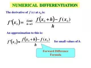
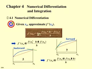
DIFFERENTIATION USING INTERPOLATION If the given tabular function y(x) is reasonably well approximated by a polynomial Pn(x) of degree n, it is hoped that the result of will also satisfactorily approximate the corresponding derivative of y(x).
However, even if Pn(x) and y(x) coincide at the tabular points, their derivatives or slopes may substantially differ at these points as is illustrated in the Figure below:
Y Pn(x) Y(x) Deviation of derivatives X Xi O
For higher order derivatives, the deviations may be even worst. However, we can estimate the error involved in such an approximation.
For non-equidistant tabular pairs (xi, yi), i = 0, …, n we can fit the data by using either Lagrange’s interpolating polynomial or by using Newton’s divided difference interpolating polynomial. In view of economy of computation, we prefer the use of the latter polynomial.
Thus, recalling the Newton’s divided difference interpolating polynomial for fitting this data as
Assuming that Pn(x) is a good approximation to y(x), the polynomial approximation to can be obtained by differentiating Pn(x). Using product rule of differentiation, the derivative of the products in Pn(x) can be seen as follows:
Thus, is approximated by which is given by
The error estimate in this approximation can be seen from the following. We have seen that if y(x) is approximated by Pn(x), the error estimate is shown to be
cannot be evaluated. However, for any of the tabular points x = xi, ∏(x) vanishes and the difficult term drops out. Thus, the error term in the last equation at the tabular point x = xi simplifies to
for some ξ in the interval I defined by the smallest and largest of x, x0, x1, …, xn and
The error in the r-th derivative at the tabular points can indeed be expressed analogously. To understand this method better, we consider the following example.
ExampleFind and from the following data using the method based on divided differences:
0.15 0.21 0.23 0.1761 0.3222 0.3617 0.27 0.32 0.35 0.4314 0.5051 0.5441
Solution We first construct divided difference table for the given data as shown below:
3rd divided difference 2nd divided difference 1st divided difference 0.1761 0.3222 0.3617 0.4314 0.5051 0.5441 0.15 0.21 0.23 0.27 0.32 0.35 2.4350 1.9750 1.7425 1.4740 1.3000 –5.7500 –3.8750 –2.9833 –2.1750 15.6250 8.1064 6.7358
Thus, using first, second and third differences from the table, the above equation yields
Therefore, Similarly, we can show that
RICHARDSON’S EXTRAPOLATION METHOD To improve the accuracy of the derivative of a function, which is computed by starting with an arbitrarily selected value of h, Richardson’s extrapolation method is often employed in practice, in the following manner:
Suppose we use two-point formula to compute the derivative of a function, then we have
where ET is the truncation error. Using Taylor’s series expansion, we can see that
The idea of Richardson’s extrapolation is to combine two computed values of using the same method but with two different step sizes usually h and h/2 to yield a higher order method. Thus, we have
Here, ci are constants, independent of h, and F(h) and F(h/2) represent approximate values of derivatives. Eliminating c1 from the above pair of equations, we get
Thus, we have obtained a fourth-order accurate differentiation formula by combining two results which are of second-order accurate. Now, repeating the above argument, we have
Eliminating d1 from the above pair of equations, we get a better approximation as
This extrapolation process can be repeated further until the required accuracy is achieved, which is called an extrapolation to the limit. Therefore the equation for F2 above can be generalized as