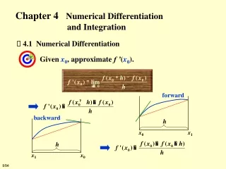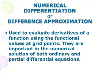
Numerical Differentiation
Numerical Differentiation. Consider a particle whose position as a function of time is recorded in a table. How do we determine its velocity v(t)=dx/dt?. Consider a particle whose position as a function of time is recorded in a table. How do we determine its velocity v(t)=dx/dt?

Numerical Differentiation
E N D
Presentation Transcript
Consider a particle whose position as a function of time is recorded in a table. How do we determine its velocity v(t)=dx/dt?
Consider a particle whose position as a function of time is recorded in a table. How do we determine its velocity v(t)=dx/dt? • We differentiate!
Consider a particle whose position as a function of time is recorded in a table. How do we determine its velocity v(t)=dx/dt? • We differentiate! • This form is not usefully as it is plagued by subtractive cancellation; h oscillates between 0 and as
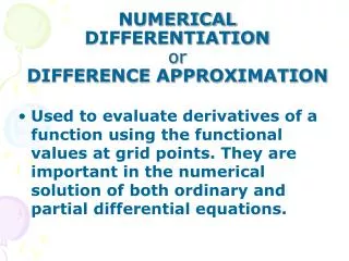
Alternative methods are the forward difference, central difference and extrapolated difference.
Alternative methods are the forward difference, central difference and extrapolated difference. • For completeness we will look very briefly at the forward difference (the other methods will be left as research).
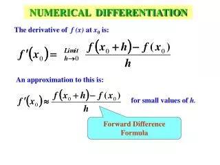
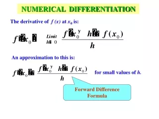
Forward Difference • This the most direct method and starts with expanding the function as a Taylor series.
Forward Difference • This the most direct method and starts with expanding the function as a Taylor series. • The series advances the function one small step forward, • h is the step size.
Forward Difference • The forward difference algorithm is obtained by solving for f prime. • Where c represents the compute value. • Ie an approx. using two points to rep the function by a straight line in the interval x to x+h
Error which is proportional to h. Forward Difference • The forward difference algorithm is obtained by solving for f prime. • Where c represents the compute value. • Ie an approx. using two points to rep the function by a straight line in the interval x to x+h
x x+h Diagram illustrating the forward difference
Forward Difference • Consider the case where,
Forward Difference • Consider the case where, • The exact derivative is • The computed derivative is • For small h the approximation becomes good. ie
Most real world problems are written as (modelled with) differential equations.
Most real world problems are written as (modelled with) differential equations. • in chemistry, physics, and engineering. • more recently in models for medicine, biology.
Most real world problems are written as (modelled with) differential equations. • in chemistry, physics, and engineering. • more recently in models for medicine, biology. • Eg. Oscillators (harmonic motion). • Assume we have a mass m attached to a spring forced by an external force.
A problem may require you to solve for the motion of the mass as a function of time.
From classical mechanics we use Newton’s 2nd law, which can be written in differential form.
From classical mechanics we use Newton’s 2nd law, which can be written in differential form. • may be used to determine v(t) and x(t) given initial conditions.
A differential equation is an equation involving an unknown function and one or more of its derivatives.
A differential equation is an equation involving an unknown function and one or more of its derivatives. • The equation is an ordinary differential equation (ODE) if the unknown function depends on only one independent variable.
Types of ordinary differential equations include initial-value problems (IVP) and boundary-value problems (BVP).
Types of ordinary differential equations include initial-value problems (IVP) and boundary-value problems (BVP). • Examplesof ODEs: Growth equation Harmonic Oscillator
The exciting feature of computational work is highlighted in that we can solve for problems of this type very easily. • We are not restricted to linear differential equations or nearly linear. There is no need for the usual common assumptions.
Linear Driven Oscillator: • Where is the force exerted by the spring and is the external force.
Linear Driven Oscillator: • Where is the force exerted by the spring and is the external force. • Nonlinear Oscillator: • PE is an arbitrary power p of displacement x from equilibrium.