GG313 Lecture 15 Eigenvectors and Eigenvalues 10/11/05
180 likes | 394 Views
GG313 Lecture 15 Eigenvectors and Eigenvalues 10/11/05. Before continuing, we covered the dot product of 2 vectors as a special case of matrix multiplication. What’s the cross product ?

GG313 Lecture 15 Eigenvectors and Eigenvalues 10/11/05
E N D
Presentation Transcript
GG313 Lecture 15 Eigenvectors and Eigenvalues 10/11/05
Before continuing, we covered the dot product of 2 vectors as a special case of matrix multiplication. What’s the cross product? If you recall your physics, the cross product of two vectors is a vector in the direction perpendicular to the plane containing the two vectors being multiplied. The amplitude of the result is the product of the input vector lengths. Classically: Where is the angle between A and B, and ||A||=Sqrt(Ax2+ Ay2 +Az2). In matrix notation:
where ji is called the unit vector in the I direction. In electronics, the induced magnetic field, the electric current and the force on a wire are related by the equation: F=I B Sin()=I x B, where F is the force, I is the electric current, and B is the magnetic field. In matrix form:
This equation describes the operation of electric motors, electric generators, mass spectrometers, and the earth’s magnetic field. If the current in a wire is described by the vector: I =[2 0 0] and the magnetic field by: B=[0 4 0], what is the strength and direction of the force exerted on the wire?
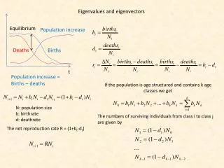
Eigenvalues and eigenvectors have their origins in physics, in particular in problems where motion is involved, although their uses extend from solutions to stress and strain problems to differential equations and quantum mechanics. Recall from last class that we used matrices to deform a body - the concept of STRAIN. Eigenvectors are vectors that point in directions where there is no rotation. Eigenvalues are the change in length of the eigenvector from the original length. **** SHOW shearstraineigen.m The basic equation in eigenvalue problems is:
(E.01) In words, this deceptively simple equation says that for the square matrix A, there is a vector x such that the product of Ax such that the result is a SCALAR, , that, when multiplied by x, results in the same product. The multiplication of vector x by a scalar constant is the same as stretching or shrinking the coordinates by a constant value.
The vector x is called an eigenvectorand the scalar , is called an eigenvalue. • Do all matrices have real eigenvalues? • No, they must be square and the determinant of A- I must equal zero. This is easy to show: • This can only be true if det(A- I )=|A- I |=0 • Are eigenvectors unique? • No, if x is an eigenvector, then x is also an eigenvector and is an eigenvalue. (E.02) (E.03) (E.04) A(x)= Ax = lx = l (x)
How do you calculate eigenvectors and eigenvalues? Expand equation (E.03): det(A- I )=|A- I |=0 for a 2x2 matrix: (E.05) For a 2-dimensional problem such as this, the equation above is a simple quadratic equation with two solutions for . In fact, there is generally one eigenvalue for each dimension, but some may be zero, and some complex.
The solution to E.05 is: (E.06) (E.07) This “characteristic equation” does not involve x, and the resulting values of can be used to solve for x. Consider the following example: Eqn. E.07 doesn’t work here because a11a22-a12a12=0, so we use E.06:
We see that one solution to this equation is =0, and dividing both sides of the above equation by yields =5. Thus we have our two eigenvalues, and the eigenvectors for the first eigenvalue, =0 are: These equations are multiples of x=-2y, so the smallest whole number values that fit are x=2, y=-1
For the other eigenvalue, =5: This example is rather special; A-1 does not exist, the two rows of A- I are dependent and thus one of the eigenvalues is zero. (Zero is a legitimate eigenvalue!) EXAMPLE: A more common case is A =[1.05 .05 ; .05 1] used in the strain exercise. Find the eigenvectors and eigenvalues for this A, and then calculate [V,D]=eig[A]. The procedure is: Compute the determinant of A- I Find the roots of the polynomial given by | A- I|=0 Solve the system of equations (A- I)x=0
Eigenvectors and eigenvalues are used in structural geology to determine the directions of principal strain; the directions where angles are not changing. In seismology, these are the directions of least compression (tension), the compression axis, and the intermediate axis (in three dimensions. Some facts: • The product of the eigenvalues=det|A| • The sum of the eigenvalues=trace(A) The x,y values of A can be thought of as representing points on an ellipse centered at 0.0. The eigenvectors are then in the directions of the major and minor axes of the ellipse, and the eigenvalues are the lengths of these axes to the ellipse from 0,0.
One particularly useful application of eigenvectors is for correlation. Recall that we can define the correlations of two functions x, and y as a correlation matrix: The correlation coefficient of x and y is 0.75. We can show this as a sort of error ellipse using the eigenvalues and eigenvectors: >> A=[1 .75;.75 1] >> [V,D]=eig(A) V = -0.7071 0.7071 0.7071 0.7071 D =0.25 0 0 1.75
We can interpret this correlation as an ellipse whose major axis is one eigenvalue and the minor axis length is the other: No correlation yields a circle, and perfect correlation yields a line.
What good are such things? Consider the matrix: What is A100 ? We can get A100 by multiplying matrices many many times: Or we could find the eigenvalues of A and obtain A100 very quickly using eigenvalues.
For now, I’ll just tell you that there are two eigenvectors for A: The eigenvectors are x1=[.6 ; .4] and x2=[1 ; -1], and the eigenvalues are 1=1 and 2=0.5. Note that if we multiply x1 by A, we get x1. If we multiply x1 by A again, we STILL get x1. Thus x1 doesn’t change as we mulitiply it by An. Don’t believe it ? - open Matlab and try it.
What about x2? When we multiply A by x2, we get x2/2, and if we multiply x2 by A2, we get x2/4 . This number gets very small fast. Note that when A is squared the eigenvectors stay the same, but the eigenvalues are squared! Back to our original problem we note that for A100, the eigenvectors will be the same, the eigenvalues 1=1 and 2=(0.5)100, which is effectively zero. Each eigenvector is multiplied by its eigenvalue whenever A is applied,