Understanding Eigenvalues and Eigenvectors in Linear Algebra
Learn the definition, computation, and solution methods for eigenvalues and eigenvectors of square matrices in Chapter 5 of Linear Algebra. Explore examples and proofs to deepen your understanding.

Understanding Eigenvalues and Eigenvectors in Linear Algebra
E N D
Presentation Transcript
Linear Algebra Chapter 5Eigenvalues and Eigenvectors 大葉大學 資訊工程系 黃鈴玲
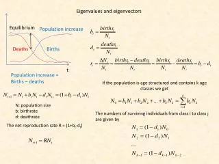
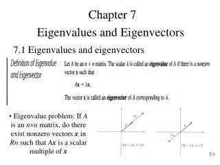
5.1 Eigenvalues and Eigenvectors Definition Let A be an n n matrix. A scalar is called an eigenvalue(特徵值,固有值)of A if there exists a nonzero vector x in Rn such that Ax = x. The vector x is called an eigenvectorcorresponding to . Figure 6.1
Computation of Eigenvalues and Eigenvectors Let A be an n n matrix with eigenvalue and corresponding eigenvector x. Thus Ax = x. This equation may be written Ax – x = 0 given (A – In)x = 0 Solving the equation |A – In| = 0 for leads to all the eigenvalues of A. On expending the determinant |A – In|, we get a polynomial in . This polynomial is called the characteristic polynomial of A. The equation |A – In| = 0 is called the characteristic equation of A.
Solution Let us first derive the characteristic polynomial of A. We get Example 1 Find the eigenvalues and eigenvectors of the matrix We now solve the characteristic equation of A. The eigenvalues of A are 2 and –1. The corresponding eigenvectors are found by using these values of in the equation(A – I2)x = 0. There are many eigenvectors corresponding to each eigenvalue.
= 2 We solve the equation (A – 2I2)x = 0 for x. The matrix (A – 2I2) is obtained by subtracting 2 from the diagonal elements of A. We get This leads to the system of equations giving x1 = –x2. The solutions to this system of equations are x1 = –r, x2 = r, where r is a scalar. Thus the eigenvectors of A corresponding to = 2 are nonzero vectors of the form
= –1 We solve the equation (A + 1I2)x = 0 for x. The matrix (A + 1I2) is obtained by adding 1 to the diagonal elements of A. We get This leads to the system of equations Thus x1 = –2x2. The solutions to this system of equations are x1 = –2s and x2 = s, where s is a scalar. Thus the eigenvectors of A corresponding to = –1 are nonzero vectors of the form 隨堂作業:9(a)先不求eigenspaces
Proof Let x1 and x2 be two vectors in the eigenspace of and let c be a scalar. Then Ax1 = x1 and Ax2 = x2. Hence, Thus is a vector in the eigenspace of . The set is closed under addition. Theorem 5.1 Let A be an n n matrix and an eigenvalue of A. The set of all eigenvectors corresponding to , together with the zero vector, is a subspace of Rn. This subspace is called the eigenspace of .
Further, since Ax1 = x1, Therefore cx1 is a vector in the eigenspace of . The set is closed scalar multiplication. Thus the set is a subspace of Rn.
Solution The matrix A – I3is obtained by subtracting from the diagonal elements of A.Thus The characteristic polynomial of A is |A – I3|. Using row and column operations to simplify determinants, we get Example 2 Find the eigenvalues and eigenvectors of the matrix
We now solving the characteristic equation of A: The eigenvalues of A are 10 and 1. The corresponding eigenvectors are found by using three values of in the equation (A – I3)x = 0.
The solution to this system of equations are x1 = 2r, x2 = 2r, and x3 = r, where r is a scalar. Thus the eigenspace of = 10 is the one-dimensional space of vectors of the form. • = 10 We get
The solution to this system of equations can be shown to be x1 = – s – t, x2 = s, and x3 = 2t, where s and t are scalars. Thus the eigenspace of = 1 is the space of vectors of the form. • = 1 Let = 1 in (A – I3)x = 0. We get
Separating the parameters s and t, we can write Thus the eigenspace of = 1 is a two-dimensional subspace of R2 with basis If an eigenvalue occurs as a k times repeated root of the characteristic equation, we say that it is of multiplicity k. Thus l=10 has multiplicity 1, while l=1 has multiplicity 2 in this example. 隨堂作業:10
Example 3 Let A be an n n matrix A with eigenvalues 1, …, n, and corresponding eigenvectors X1, …, Xn. Prove that if c 0, then the eigenvalues of cA are c1, …, cn with corresponding eigenvectors X1, …, Xn. 隨堂作業:28 Solution Let i be one of eigenvalues of A with corresponding eigenvectors Xi. Then AXi = iXi. Multiply both sides of this equation by c to get cAXi = ciXi Thus ci is an eigenvalues of cA with corresponding eigenvector Xi. Further, since cA is n n matrix, the characteristic polynomial of A is of degree n. The characteristic equation has n roots, implying that cA has n eigenvalues. The eigenvalues of cA are therefore c1, …, cn with corresponding eigenvectors X1, …, Xn.
Homework • Exercise 5.1:9, 10, 13, 15, 24, 26, 32 Ex24: Prove that if A is a diagonal matrix, then its eigenvalues are the diagonal elements. Ex26: Prove that if A and Athave the same eigenvalues. Ex32: Prove that the constant term of the characteristic polynomial of a matrix A is |A|.
5.3 Diagonalization of Matrices Definition Let A and B be square matrices of the same size. B is said to be similar to A if there exists an invertible matrix C such that B = C–1AC. The transformation of the matrix A into the matrix B in this manner is called a similarity transformation.
Example 1 Consider the following matrices A and C. C is invertible. Use the similarity transformation C–1AC to transform A into a matrix B. Solution 隨堂作業:1(b)
Theorem 5.3 Similar matrices have the same eigenvalues. Proof Let A and B be similar matrices. Hence there exists a matrix C such that B = C–1AC. The characteristic polynomial of B is |B – In|. Substituting for B and using the multiplicative properties of determinants, we get The characteristic polynomials of A and B are identical. This means that their eigenvalues are the same.
Theorem 5.4 • Let A be an n n matrix. • If A has n linearly independent eigenvectors, it is diagonalizable. The matrix C whose columns consist of n linearly independent eigenvectors can be used in a similarity transformation C–1AC to give a diagonal matrix D. The diagonal elements of D will be the eigenvalues of A. • If A is diagonalizable, then it has n linearly independent eigenvectors Definition A square matrixA is said to be diagonalizable if there exists a matrix C such that D = C–1AC is a diagonal matrix.
Proof (a) Let A have eigenvalues 1, …, n, with corresponding linearly independent eigenvectors v1, …, vn. Let C be the matrix having v1, …, vn as column vectors. C = [v1 … vn] Since Av1 = 1v1, …, Avn = 1vn, matrix multiplication in terms of columns gives
Since the columns of C are linearly independent, C is nonsingular. Thus Therefore, if an n n matrix A has n linearly independent eigenvectors, these eigenvectors can be used as the columns of a matrix A that diagonalizes A. The diagonal matrix has the eigenvaules of A as diagonal elements.
(b) The converse is proved by retracting the above steps. Commence with the assumption that C is a matrix [v1 … vn] that diagonalizes A. Thus, there exist scalars 1, …, n, such that Retracting the above steps, we arrive at the conclusion that Av1 = 1v1, …, Avn = nvn The v1, …, vn are eigenvectors of A. Since C is nonsingular, these vectors (column vectors of C) are linearly independent. Thus if an n n matrix A is diagonalizable, it has n linearly independent eigenvectors.
The eigenvalues and corresponding eigenvector of this matrix were found in Example 1 of Section 5.1. They are • Since A, a 2 2 matrix, has two linearly independent eigenvectors, it is diagonalizable. Example 2 • Show that the following matrix A is diagonalizable. • Find a diagonal matrix D that is similar to A. • Determine the similarity transformation that diagonalizes A. Solution
(b) A is similar to the diagonal matrix D, which has diagonal elements 1 = 2 and 2 = –1. Thus (c) Select two convenient linearly independent eigenvectors, say Let these vectors be the column vectors of the diagonalizing matrix C. We get 隨堂作業:3(a)
Note If A is similar to a diagonal matrix D under the transformation C–1AC, then it can be shown that Ak = CDkC–1. This result can be used to compute Ak. Let us derive this result and then apply it. This leads to
A is the matrix of the previous example. Use the values of C and D from that example. We get Example 3 Compute A9 for the following matrix A. Solution 隨堂作業:9(a)
The characteristic equation is There is a single eigenvalue, = 2. We find the corresponding eigenvectors. (A – 2I2)x = 0 gives Thus x1 = r, x2 = r. The eigenvectors are nonzero vectors of the form The eigenspace is a one-dimensional space. A is a 2 2 matrix, but it does not have two linearly independent eigenvectors. Thus A is not diagonalizable. Example 4 Show that the following matrix A is not diagonalizable. Solution 隨堂作業:3(c)
Orthogonal Diagonalization Definition A square matrix A is said to be orthogonally diagonalizable if there exists an orthogonal matrix C such that D = C-1AC is a diagonal matrix. Theorem 5.5 • Let A be an n n symmetric matrix. • All the eigenvalues of A are real numbers. • The dimensional of an eigenspace of A is the multiplicity of the eigenvalues as a root of the characteristic equation. • The eigenspaces of A are orthogonal. • A has n linearly independent eigenvectors.
Example 5 Orthogonally diagonalize the following symmetric matrix A. Solution The eigenvalues and corresponding eigenspaces of this matrix are Theorem 5.6 Let A be a square matrix. A is orthogonally diagonalizable if and only if it is a symmetric matrix.
Since A is symmetric, it can be diagonalized to give Let us determine the transformation. The eigenspaces V1 and V2 are orthogonal. Use a unit vector in each eigenspace as columns of an orthogonal matrix C. We get The orthogonal transformation that leads to D is 隨堂作業:6(a)
Homework • Exercise 5.3:1, 2, 6, 9