Berthing Problem
Berthing Problem. Chen Fang Yew Nicholas 1 , Gani Zhi Hao Terry 1 , Vo Thanh Minh Tue 1 1 NUS High School of Mathematics and Science, Singapore. Introduction. The given problem is very complex and arises in daily management of the Port of Singapore .


Berthing Problem
E N D
Presentation Transcript
Berthing Problem Chen Fang Yew Nicholas1, Gani Zhi Hao Terry1, Vo Thanh Minh Tue1 1NUS High School of Mathematics and Science, Singapore
Introduction • The given problem is very complex and arises in daily management of the Port of Singapore. • The port success depends on a robust and efficient berthing plan. • The program must compute on demand.
Introduction • We propose a greedy first fit algorithm to solve the berthing problem. • We also introduce graph theory as a possible approach to solve the problem.
The problem • Ships arrive at various times and have different lengths and berthing times. • Our task is to devise a berthing plan that minimizes the waiting time for all ships.
Objective • Minimize the waiting time function • Where is the time the ship is berthed, Is the arrival time, and is the waiting constant
Wait time case study • When =1, LHS=RHS • Either order is the same.
Wait time case study • Second option incurs more waiting time • Minimizing total height equates to minimizing total j, waiting time. • First fit algorithm.
First fit algorithm • Greedy algorithm. • Choose the lowest time possible. • Choose the lowest space possible.
Advantages • Extremely fast to compute. • Give a reasonable good solution. • Modify the algorithm to meet realistic constraints.
Modified realistic algorithm • “port stay times are often delayed beyond the estimated values” • Takes into account delay time • Models after realistic conditions • Allows for inter-clearance distance between ships
Discretization • Transform continuous data into discrete values. • Simplify the data input. • Scale the solution range.
A novel approach • Apply graph theory. • Rigorous mathematical ground.
Berthing problem • Variables • ai: Arrival time of ith ship. • hi: Processing time. • Li: Length of the ship. • Waiting penalty for ith ship: (yi – ai )α
Berthing problem • Solution: { (t1, y1), (t2, y2), …, (tn, yn) } • ti: Time in which ith ship starts to dock. • yi : Lower y-coordinate of ith ship. • Objective function.
Solution space • (ti, yi) • Every point in a solution space is a feasible solution. • Overlapping of solution spaces yields solution domain.
Solution space • Overlapping of rectangle <=> incompatible solution pairs. • Compatible solution pairs. • (ti, yi) (tj, yj)
Graph theory • Each solution (ti, yi, i) can be assigned as a vertex. • Compatible solutions are joined by an edge. Vertex for ith ship: (ti, yi) E = (ti – ai)α + (tj – aj)α Vertex for jth ship: (tj, yj)
Graph theory • Consider six ships A to F with solution pairs SA to SF • The vertices A to F and their edges form a complete graph • A cycle is created as all the vertices join to each other once. AF A F AB EF E B BC DE CD D C
Graph theory • By adding the weight of each edge of the cycle together, the overall delay time can be calculated.
Graph theory • A swap in position of vertices within the cycle does not change the overall delay time. AF AF A F F A AB BF EF AE = E E B B BC DE BC DE CD CD
Graph theory • Consider another vertex not within the cycle • If weight of new edge < weight of old edge, replace old vertex with new vertex AF A F FG AB EF G E B BC DE DG CD
Graph theory • For example, • If wFG + wDG < wEF + wDE, then replace E with G AF A F FG AB EF G E B BC DE DG CD
The algorithm • Start with the earliest ship. • Depth-first-search for a possible complete sub graph. • Check all vertices in the graph if improvement possible. • If no improvement possible, then the program terminates.
Advantages • Greedy algorithm can give a reasonable good solution. • By transforming from a geometrical problem to a graph problem, we can handle constraints more easily.
Challenges • Large number of vertices and edges. • Complex relationship.
Conclusion • Justified using first fit algorithm • Devised an algorithm to solve the problem • Improved on it to take into account realistic conditions • Suggested a novel approach using graph theory to solve this problem
References • Dai, J., Lin, W., Moorthy, R., & Teo, C.-P. (2003). Berth Allocation Planning Optimization in Container Terminal. 1-33. • Duin, C. W., & Sluis, E. v. (n.d.). On the complexity of Adjacent Resource Scheduling. • Lim, A. (n.d.). An Effective Ship Berthing Algorithm.
The end • Thank you for your attention.