Strip-Plot Designs
Strip-Plot Designs. Sometimes called split-block design For experiments involving factors that are difficult to apply to small plots Three sizes of plots so there are three experimental errors The interaction is measured with greater precision than the main effects. S3 S1 S2.

Strip-Plot Designs
E N D
Presentation Transcript
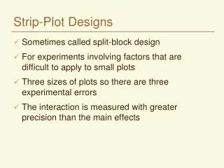
Strip-Plot Designs • Sometimes called split-block design • For experiments involving factors that are difficult to apply to small plots • Three sizes of plots so there are three experimental errors • The interaction is measured with greater precision than the main effects
S3 S1 S2 S1 S3 S2 N1 N2 N0 N3 N2 N3 N1 N0 For example: • Three seed-bed preparation methods • Four nitrogen levels • Both factors will be applied with large scale machinery
Advantages --- Disadvantages • Advantages • Permits efficient application of factors that would be difficult to apply to small plots • Disadvantages • Differential precision in the estimation of interaction and the main effects • Complicated statistical analysis
Strip-Plot Analysis of Variance Source df SS MS F Total rab-1 SSTot Block r-1 SSR MSR A a-1 SSA MSA FA Error(a) (r-1)(a-1) SSEA MSEAFactor A error B b-1 SSB MSB FB Error(b) (r-1)(b-1) SSEB MSEBFactor B error AB (a-1)(b-1) SSAB MSAB FAB Error(ab) (r-1)(a-1)(b-1) SSEAB MSEABSubplot error
Computations • There are three error terms - one for each main plot and interaction plot SSTot SSR SSA SSEA SSB SSEB SSAB SSEAB SSTot-SSR-SSA-SSEA-SSB-SSEB-SSAB
F Ratios • F ratios are computed somewhat differently because there are three errors • FA = MSA/MSEAtests the sig. of the A main effect • FB = MSB/MSEBtests the sig. of the B main effect • FAB = MSAB/MSEABtests the sig. of the AB interaction
Standard Errors of Treatment Means • Factor A Means MSEA/rb • Factor B Means MSEB/ra • Treatment AB Means MSEAB/r
SE of Differences • Differences between 2 A means 2MSEA/rb • Differences between 2 B means 2MSEB/ra • Differences between A means at same level of B 2[(b-1)MSEAB + MSEA]/rb • Difference between B means at same level of A 2[(a-1)MSEAB + MSEB]/ra • Differences between A and B means at diff. levels 2[(ab-a-b)MSEAB + (a)MSEA + (b)MSEB]/rab For se that are calculated from >1 MSE, df are approximated
Interpretation Much the same as a two-factor factorial: • First test the AB interaction • If it is significant, the main effects have no meaning even if they test significant • Summarize in a two-way table of AB means • If AB interaction is not significant • Look at the significance of the main effects • Summarize in one-way tables of means for factors with significant main effects
Numerical Example • A pasture specialist wanted to determine the effect of phosphorus and potash fertilizers on the dry matter production of barley to be used as a forage • Potash: K1=none, K2=25kg/ha, K3=50kg/ha • Phosphorus: P1=25kg/ha, P2=50kg/ha • Three blocks • Farm scale fertilization equipment
K3 K1 K2 P1 56 32 49 P2 67 54 58 K1 K3 K2 P2 38 62 50 P1 52 72 64 K2 K1 K3 P2 54 44 51 P1 63 54 68
Raw data - dry matter yields Treatment I II III P1K1 32 52 54 P1K2 49 64 63 P1K3 56 72 68 P2K1 54 38 44 P2K2 58 50 54 P2K3 67 62 51
Construct two-way tables Phosphorus x Block P I II III Mean 1 45.67 62.67 61.67 56.67 2 59.67 50.00 49.67 53.11 Mean 52.67 56.33 55.67 54.89 Potash x Block K I II III Mean 1 43.0 45.0 49.0 45.67 2 53.5 57.0 58.5 56.33 3 61.5 67.0 59.5 62.67 Mean 52.67 56.33 55.67 54.89 Potash x Phosphorus P K1 K2 K3 Mean 1 46.00 58.67 65.33 56.67 2 45.33 54.00 60.00 53.11 Mean 45.67 56.33 62.67 54.89
ANOVA Source df SS MS F Total 17 1833.78 Block 2 45.78 22.89 Potash (K) 2 885.78 442.89 22.64** Error(a) 4 78.22 19.56 Phosphorus (P) 1 56.89 56.89 .16ns Error(b) 2 693.78 346.89 KxP 2 19.11 9.56 .71ns Error(ab) 4 54.22 13.55
Raw data - dry matter yields Treatment I II III P1K1 32 52 54 P1K2 49 64 63 P1K3 56 72 68 P2K1 54 38 44 P2K2 58 50 54 P2K3 67 72 51 SSTot=devsq(range)
ANOVA Source df SS MS F Total 17 1833.78
Construct two-way tables Phosphorus x Block Potash x Block P I II III Mean 1 45.67 62.67 61.67 56.67 2 59.67 50.00 49.67 53.11 Mean 52.67 56.33 55.67 54.89 K I II III Mean 1 43.0 45.0 49.0 45.67 2 53.5 57.0 58.5 56.33 3 61.5 67.0 59.5 62.67 Mean 52.67 56.33 55.67 54.89 Potash x Phosphorus P K1 K2 K3 Mean 1 46.00 58.67 65.33 56.67 2 45.33 54.00 60.00 53.11 Mean 45.67 56.33 62.67 54.89 Sums of Squares for Blocks SSR=6*devsq(range)
ANOVA Source df SS MS F Total 17 1833.78 Block 2 45.78 22.89
Construct two-way tables Phosphorus x Block Potash x Block P I II III Mean 1 45.67 62.67 61.67 56.67 2 59.67 50.00 49.67 53.11 Mean 52.67 56.33 55.67 54.89 K I II III Mean 1 43.0 45.0 49.0 45.67 2 53.5 57.0 58.5 56.33 3 61.5 67.0 59.5 62.67 Mean 52.67 56.33 55.67 54.89 Potash x Phosphorus P K1 K2 K3 Mean 1 46.00 58.67 65.33 56.67 2 45.33 54.00 60.00 53.11 Mean 45.67 56.33 62.67 54.89 Main effect of Potash SSA=6*devsq(range)
ANOVA Source df SS MS F Total 17 1833.78 Block 2 45.78 22.89 Potash 2 885.78 442.89
Construct two-way tables Phosphorus x Block Potash x Block P I II III Mean 1 45.67 62.67 61.67 56.67 2 59.67 50.00 49.67 53.11 Mean 52.67 56.33 55.67 54.89 K I II III Mean 1 43.0 45.0 49.0 45.67 2 53.5 57.0 58.5 56.33 3 61.5 67.0 59.5 62.67 Mean 52.67 56.33 55.67 54.89 Potash x Phosphorus P K1 K2 K3 Mean 1 46.00 58.67 65.33 56.67 2 45.33 54.00 60.00 53.11 Mean 45.67 56.33 62.67 54.89 SSEA =2*devsq(range) – SSR – SSA
ANOVA Source df SS MS F Total 17 1833.78 Block 2 45.78 22.89 Potash 2 885.78 442.89 22.64** Error(a) 4 78.22 19.56
Construct two-way tables Phosphorus x Block Potash x Block P I II III Mean 1 45.67 62.67 61.67 56.67 2 59.67 50.00 49.67 53.11 Mean 52.67 56.33 55.67 54.89 K I II III Mean 1 43.0 45.0 49.0 45.67 2 53.5 57.0 58.5 56.33 3 61.5 67.0 59.5 62.67 Mean 52.67 56.33 55.67 54.89 Potash x Phosphorus P K1 K2 K3 Mean 1 46.00 58.67 65.33 56.67 2 45.33 54.00 60.00 53.11 Mean 45.67 56.33 62.67 54.89 Main effect of Phosphorous SSB=9*devsq(range)
ANOVA Source df SS MS F Total 17 1833.78 Block 2 45.78 22.89 Potash 2 885.78 442.89 22.64** Error(a) 4 78.22 19.56 Phosphorus 1 56.89 56.89
Construct two-way tables Phosphorus x Block Potash x Block P I II III Mean 1 45.67 62.67 61.67 56.67 2 59.67 50.00 49.67 53.11 Mean 52.67 56.33 55.67 54.89 K I II III Mean 1 43.0 45.0 49.0 45.67 2 53.5 57.0 58.5 56.33 3 61.5 67.0 59.5 62.67 Mean 52.67 56.33 55.67 54.89 Potash x Phosphorus P K1 K2 K3 Mean 1 46.00 58.67 65.33 56.67 2 45.33 54.00 60.00 53.11 Mean 45.67 56.33 62.67 54.89 SSEB =3*devsq(range) – SSR – SSB
ANOVA Source df SS MS F Total 17 1833.78 Block 2 45.78 22.89 Potash 2 885.78 442.89 22.64** Error(a) 4 78.22 19.56 Phosphorus 1 56.89 56.89 .16ns Error(b) 2 693.78 346.89
Construct two-way tables Phosphorus x Block Potash x Block P I II III Mean 1 45.67 62.67 61.67 56.67 2 59.67 50.00 49.67 53.11 Mean 52.67 56.33 55.67 54.89 K I II III Mean 1 43.0 45.0 49.0 45.67 2 53.5 57.0 58.5 56.33 3 61.5 67.0 59.5 62.67 Mean 52.67 56.33 55.67 54.89 Potash x Phosphorus P K1 K2 K3 Mean 1 46.00 58.67 65.33 56.67 2 45.33 54.00 60.00 53.11 Mean 45.67 56.33 62.67 54.89 Interaction of P and K SSAB=3*devsq(range) – SSA – SSB
ANOVA Source df SS MS F Total 17 1833.78 Block 2 45.78 22.89 Potash (K) 2 885.78 442.89 22.64** Error(a) 4 78.22 19.56 Phosphorus (P) 1 56.89 56.89 .16ns Error(b) 2 693.78 346.89 KxP 2 19.11 9.56 .71ns Error(ab) 4 54.22 13.55
Interpretation • Only potash had a significant effect • Each increment of added potash resulted in an increase in the yield of dry matter • The increase took place regardless of the level of phosphorus Potash None 25 kg/ha 50 kg/ha SE Mean Yield 45.67 56.33 62.67 1.80
Repeated measurements over time • We often wish to take repeated measures on experimental units to observe trends in response over time. • repeated cuttings of a pasture • multiple observations on the same animal (developmental responses) • Often provides more efficient use of resources than using different experimental units for each time period • May also provide more precise estimation of time trends by reducing random error among experimental units – effect is similar to blocking • Problem: observations over time are not assigned at random to experimental units. • Observations on the same plot will tend to be positively correlated • Correlations are greatest for samples taken at short time intervals and less for distant sampling periods
Repeated measurements over time • The simplest approach is to treat sampling times as sub-plots in a split-plot experiment. • Some references recommend use of strip-plot rather than split-plot • This is valid only if all pairs of sub-plots in each main plot can be assumed to be equally correlated. • Compound symmetry • Sphericity • Univariate adjustments can be made • Multivariate procedures can be used to adjust for the correlations among sampling periods
Univariate adjustments for repeated measures • Reduce df for subplots, interactions, and subplot error terms to obtain more conservative F tests • Fit a smooth curve to the time trends and analyze a derived variable • average • maximum response • area under curve • time to reach the maximum • Use polynomial contrasts to evaluate trends over time (linear, quadratic responses) and compare responses for each treatment • Can be done with the REPEATED statement in PROC GLM
Multivariate adjustments for repeated measures • Stage one: estimate covariance structure for residuals • Stage two: • include covariance structure in the model • use generalized least squares methodology to evaluate treatment and time effects • Computer intensive • use PROC MIXED or GLIMMIX in SAS Reference: Littell et al., 2002. SAS for Linear Models, Chapter 8.