Split-Plot Designs
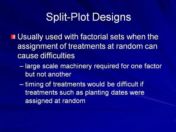
Split-Plot Designs. Usually used with factorial sets when the assignment of treatments at random can cause difficulties large scale machinery required for one factor but not another irrigation tillage plots that receive the same treatment must be grouped together

Split-Plot Designs
E N D
Presentation Transcript
Split-Plot Designs • Usually used with factorial sets when the assignment of treatments at random can cause difficulties • large scale machinery required for one factor but not another • irrigation • tillage • plots that receive the same treatment must be grouped together • for a treatment such as planting date, it may be necessary to group treatments to facilitate field operations • in a growth chamber experiment, some treatments must be applied to the whole chamber (light regime, humidity, temperature), so the chamber becomes the main plot
Different size requirements • The split plot is a design which allows the levels of one factor to be applied to large plots while the levels of another factor are applied to small plots • Large plots are whole plots or main plots • Smaller plots are split plots or subplots
Randomization • Levels of the whole-plot factor are randomly assigned to the main plots, using a different randomization for each block (for an RBD) • Levels of the subplots are randomly assigned within each main plot using a separate randomization for each main plot A2 A1 A3 Main Plot Factor Sub-Plot Factor B2 B4 B1 B3 One Block
Randomizaton Block I T3 T1 T2 V3 V4 V2 V1 V1 V4 V2 V3 V3 V4 V2 V1 Block II T1 T3 T2 V1 V2 V3 V3 V1 V4 V2 V3 V1 V4 V4 V2 Tillage treatments are main plots Varieties are the subplots
Experimental Errors • Because there are two sizes of plots, there are two experimental errors - one for each size plot • Usually the sub-plot error is smaller and has more degrees of freedom • Therefore the main plot factor is estimated with less precision than the subplot and interaction effects • Precision is an important consideration in deciding which factor to assign to the main plot
Advantages • Permits the efficient use of some factors that require different sizes of plot for their application • Permits the introduction of new treatments into an experiment that is already in progress
Disadvantages • Main plot factor is estimated with less precision so larger differences are required for significance – may be difficult to obtain adequate degrees of freedom for the main plot error • Statistical analysis is more complex because different standard errors are required for different comparisons
Uses • In experiments where different factors require different size plots • To introduce new factors into an experiment that is already in progress
Data Analysis • This is a form of a factorial experiment so the analysis is handled in much the same manner • We will estimate and test the appropriate main effects and interactions • Analysis proceeds as follows: • Construct tables of means • Complete an analysis of variance • Perform significance tests • Compute means and standard errors • Interpret the analysis
Split-Plot Analysis of Variance Source df SS MS F Total rab-1 SSTot Block r-1 SSR MSR FR A a-1 SSA MSA FA Error(a) (r-1)(a-1) SSEA MSEAMain plot error B b-1 SSB MSB FB AB (a-1)(b-1) SSAB MSAB FAB Error(b) a(r-1)(b-1) SSEB MSEBSubplot error
Computations • Only the error terms are different from the usual two- factor analysis SSTot SSR SSA SSEA SSB SSAB SSEBSSTot - SSR - SSA - SSEA - SSB - SSAB
F Ratios • F ratios are computed somewhat differently because there are two errors • FR=MSR/MSEAtests the effectiveness of blocking • FA=MSA/MSEAtests the sig. of the A main effect • FB=MSB/MSEBtests the sig. of the B main effect • FAB=MSAB/MSEBtests the sig. of the AB interaction
Standard Errors of Treatment Means • Factor A Means • Factor B Means • Treatment AB Means
SE of Differences • Differences between 2 A means with (r-1)(a-1) df • Differences between 2 B meanswith a(r-1)(b-1) df • Differences between B means at same level of A e.g., YA1B1‒ YA1B2 with a(r-1)(b-1) df • Difference between A means at same or different level of B e.g., YA1B1‒ YA2B1 or YA1B1‒ YA2B2 critical tA has (r-1)(a-1) df critical tBhas a(r-1)(b-1) df use critical t’ to compare means
Interpretation Much the same as a two-factor factorial: • First test the AB interaction • If it is significant, the main effects have no meaning even if they test significant • Summarize in a two-way table of AB means • If AB interaction is not significant • Look at the significance of the main effects • Summarize in one-way tables of means for factors with significant main effects
For example: • A wheat breeder wanted to determine the effect of planting date on the yield of four varieties of winter wheat • Two factors: • Planting date (Oct 15, Nov 1, Nov 15) • Variety (V1, V2, V3, V4) • Because of the machinery involved, planting dates were assigned to the main plots • Used a Randomized Block Design with 3 blocks
Split plot Factorial in RBD Comparison with conventional RBD • With a split-plot, there is better precision for sub-plots than for main plots, but neither has as many error df as with a conventional factorial • There may be some gain in precision for subplots and interactions from having all levels of the subplots in close proximity to each other
BlockIIIIII D1 D2 D3 D1 D2 D3 D1 D2 D3 Variety 1 25 30 17 31 32 20 28 28 19 Variety 2 19 24 20 14 20 16 16 24 20 Variety 3 22 19 12 20 18 17 17 16 15 Variety 4 11 15 8 14 13 13 14 19 8 Raw Data
Construct two-way tables Date I II III Mean 1 19.25 19.75 18.75 19.25 2 22.00 20.75 21.75 21.50 3 14.25 16.50 15.50 15.42 Mean 18.50 19.00 18.67 18.72 Block x Date Means Date V1 V2 V3 V4 Mean 1 28.00 16.33 19.67 13.00 19.25 2 30.00 22.67 17.67 15.67 21.50 3 18.67 18.67 14.67 9.67 15.42 Mean 25.56 19.22 17.33 12.78 18.72 Variety x Date Means
ANOVA Source df SS MS F Total 35 1267.22 Block 2 1.55 .78 0.22 Date 2 227.05 113.53 32.16** Error (a) 4 14.12 3.53 Variety 3 757.89 252.63 37.82** Var x Date 6 146.28 24.38 3.65* Error (b) 18 120.33 6.68
Report and Summarization Variety Date 1 2 3 4 Mean Oct 15 28.00 16.33 19.67 13.00 19.25 Nov 1 30.00 22.67 17.67 15.67 21.50 Nov 15 18.67 18.67 14.67 9.67 15.42 Mean 25.55 19.22 17.33 12.78 18.72 Standard errors: Date=0.542; Variety=0.862; Variety x Date=1.492
Interpretation • Differences among varieties depended on planting date • Even so, variety differences and date differences were highly significant • Except for variety 3, each variety produced its maximum yield when planted on November 1 • On the average, the highest yield at every planting date was achieved by variety 1 • Variety 4 produced the lowest yield for each planting date
Visualizing Interactions 30 V1 25 V2 20 Mean Yield (kg/plot) V3 15 V4 10 5 1 2 3 Planting Date
Variations • Split-plot arrangement of treatments could be used in a CRD or Latin Square, as well as in an RBD • Could extend the same principles to include another factor in a split-split plot (3-way factorial) • Could add another factor without an additional split (3-way factorial, split-plot arrangement of treatments) • ‘axb’ main plots and ‘c’ sub-plots or • ‘a’ main plots and ‘bxc’ sub-plots

