Parallel Computer Models
Parallel Computer Models. CEG 4131 Computer Architecture III Miodrag Bolic. Overview. Flynn’s taxonomy Classification based on the memory arrangement Classification based on communication Classification based on the kind of parallelism Data-parallel Function-parallel . Flynn’s Taxonomy.

Parallel Computer Models
E N D
Presentation Transcript
Parallel Computer Models CEG 4131 Computer Architecture III Miodrag Bolic
Overview • Flynn’s taxonomy • Classification based on the memory arrangement • Classification based on communication • Classification based on the kind of parallelism • Data-parallel • Function-parallel
Flynn’s Taxonomy – The most universally excepted method ofclassifying computer systems – Published in the Proceedings of the IEEE in1966 – Any computer can be placed in one of 4 broadcategories » SISD: Single instruction stream, singledata stream » SIMD: Single instruction stream, multipledata streams » MIMD: Multiple instruction streams,multiple data streams » MISD: Multiple instruction streams, singledata stream
SISD Instructions Processing element (PE) Main memory (M) Data IS DS IS Control Unit PE PE Memory
SIMD • Applications: • Image processing • Matrix manipulations • Sorting
SIMD Architectures • Fine-grained • Image processing application • Large number of PEs • Minimum complexity PEs • Programming language is a simple extension of a sequential language • Coarse-grained • Each PE is of higher complexity and it is usually built with commercial devices • Each PE has local memory
MISD • Applications: • Classification • Robot vision
Flynn taxonomy – Advantages of Flynn » Universally accepted » Compact Notation » Easy to classify a system (?) – Disadvantages of Flynn » Very coarse-grain differentiation amongmachine systems » Comparison of different systems is limited » Interconnections, I/O, memory notconsidered in the scheme
Classification based on memory arrangement Shared memory Interconnectionnetwork Interconnectionnetwork I/O1 I/On PE1 PEn M1 Mn PE1 PEn Processors P1 Pn Shared memory - multiprocessors Message passing - multicomputers
Shared-memory multiprocessors • Uniform Memory Access (UMA) • Non-Uniform Memory Access (NUMA) • Cache-only Memory Architecture (COMA) • Memory is common to all the processors. • Processors easily communicate by means of shared variables.
P P n 1 $ $ Inter connection network Mem Mem The UMA Model • Tightly-coupled systems (high degree of resource sharing) • Suitable for general-purpose and time-sharing applications by multiple users.
Symmetric and asymmetric multiprocessors • Symmetric: - all processors have equal access to all peripheral devices.- all processors are identical. • Asymmetric:- one processor (master) executes theoperating system- other processors may be of different types and may be dedicated to special tasks.
The NUMA Model • The access time varies with the location of the memory word. • Shared memory is distributed to local memories. • All local memories form a global address space accessible by all processors Access time: Cache, Local memory, Remote memory COMA - Cache-only Memory Architecture P P n 1 $ $ Mem Mem Inter connection network Distributed Memory (NUMA)
Distributed memory multicomputers • Multiple computers- nodes • Message-passing network • Local memories are private with its own program and data • No memory contention so that the number of processors is very large • The processors are connected by communication lines, and the precise way in which the lines are connected is called the topology of the multicomputer. • A typical program consists of subtasks residing in all the memories. M M M PE PE PE Interconnectionnetwork PE PE PE M M M
Classification based on type of interconnections • Static networks • Dynamic networks
Interconnection Network [1] • Mode of Operation (Synchronous vs. Asynchronous) • Control Strategy (Centralized vs. Decentralized) • Switching Techniques (Packet switching vs. Circuit switching) • Topology (Static Vs. Dynamic)
Classification based on the kind of parallelism[3] Parallel architectures PAs Data-parallel architectures Function-parallel architectures Instruction-level PAs Thread-level PAs Process-level PAs DPs ILPS MIMDs Pipelined Superscalar Ditributed Shared Vector Associative Systolic SIMDs VLIWs memory memory processors and neural architecture processors architecture MIMD (multi- architecture (multi-computer) Processors)
References • Advanced Computer Architecture and Parallel Processing, by Hesham El-Rewini and Mostafa Abd-El-Barr, John Wiley and Sons, 2005. • Advanced Computer Architecture Parallelism, Scalability, Programmability, by K. Hwang, McGraw-Hill 1993. • Advanced Computer Architectures – A Design Space Approach by Desco Sima, Terence Fountain and Peter Kascuk, Pearson, 1997.
Speedup • S = Speed(new) / Speed(old) • S = Work/time(new) / Work/time(old) • S = time(old) / time(new) • S = time(before improvement) / time(after improvement)
Speedup • Time (one CPU): T(1) • Time (n CPUs): T(n) • Speedup: S • S = T(1)/T(n)
Amdahl’s Law The performance improvement to be gained from using some faster mode of execution is limited by the fraction of the time the faster mode can be used
Example 20 hours B A must walk 200 miles Walk 4 miles /hour Bike 10 miles / hour Car-1 50 miles / hour Car-2 120 miles / hour Car-3 600 miles /hour
Example 20 hours B A must walk 200 miles Walk 4 miles /hour 50 + 20 = 70 hours S = 1 Bike 10 miles / hour 20 + 20 = 40 hours S = 1.8 Car-1 50 miles / hour 4 + 20 = 24 hours S = 2.9 Car-2 120 miles / hour 1.67 + 20 = 21.67 hours S = 3.2 Car-3 600 miles /hour 0.33 + 20 = 20.33 hours S = 3.4
Amdahl’s Law (1967) • : The fraction of the program that is naturally serial • (1- ): The fraction of the program that is naturally parallel
S = T(1)/T(N) T(1)(1- ) T(N) = T(1) + N 1 N S = = (1- ) + N + (1- ) N