Download
1 / 51
620 likes | 977 Views
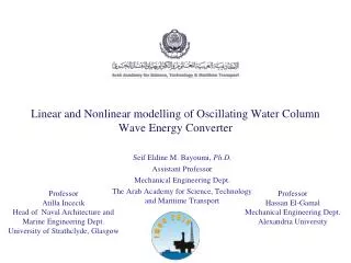
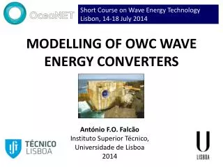
Short Course on Wave Energy Technology Lisbon, 14-18 July 2014. MODELLING OF OWC WAVE ENERGY CONVERTERS. António F.O. Falcão Instituto Superior Técnico, Universidade de Lisboa 2014. Basic approaches to OWC modelling. will be analized here. Basic equations.

E N D
Short Course on Wave Energy Technology Lisbon, 14-18 July 2014 MODELLING OF OWC WAVE ENERGY CONVERTERS António F.O. Falcão Instituto Superior Técnico, Universidade de Lisboa 2014
Basic approaches to OWC modelling will be analized here
Basic equations Volume flow rate of air displaced by OWC motion • Decomposeinto • excitationflow rate • radiationflow rate
Thermodynamics of air chamber Assume compression/decompression process in air chamber to be isentropic (adiabatic + reversible)
Aerodynamics of air turbine X X Dependence on Mach number Ma in general neglected, because of scarce information from model testing.
Frequency domain analysis • Linear turbine • Linear relationship air density versus pressure Linearize: Wells turbine
Frequency domain analysis The system is linear Decompose Note: radiation conductance G cannot be negative
Frequency domain analysis (deep water) Axisymmetric body (deep water)
Frequency domain analysis Power Power available to turbine = pressure head x volume flow rate Regular waves Time average
Frequency domain analysis Power Turbine power output Wells turbine
Exercise Compute the turbine power ouput of the Pico OWC plant, for regular waves of period 10 s and amplitude 1.0 m. The diameter of the turbine rotor is 2.3 m. The maximum alowable rotational speed is about 1500 rpm.
Frequency domain analysis Dimensional analysis
Model testing: similarity laws for air chamber and air turbine Correct dynamic similarity requires all terms in equation to take equal values in similar conditions at model size 1 and full size 2 . 1 2 air chamber
Turbine dimensionless parameters (representing the turbine aerodynamic performance) take equal values for similar conditions of the air pressure cycle in the chamber of the model and the full-sized converter. We take such conditions as those of maximum air pressure . Turbine size Turbine rotational speed The two turbines are geometrically similar
Time-domain analysis of OWCs The Wells turbine is approximately linear. So frequency-domain analysis is a good approximation. Other turbines (e.g. impulse turbines) are far from linear. So, time-domain analysis must be used, even in regular waves. This affects specially the radiation flow rate, with memory effects. The theoretical approach is similar to time-domain analysis of oscillating bodies.
radiation flow rate memory function
Introduction Theoretical/numerical hydrodynamic modelling • Frequency-domain • Time-domain • Stochastic In all cases, linear water wave theory is assumed: • small amplitude waves and small body-motions • real viscous fluid effects neglected Non-linear water wave theory and CFD may be used at a later stage to investigate some water flow details.
Introduction Frequency domain model Basic assumptions: • Monochromatic (sinusoidal) waves • The system (input output) is linear (e.g. a linear damper and a linear spring) • Historically the first model • The starting point for the other models Advantages: • Easy to model and to run • First step in optimization process • Provides insight into device’s behaviour Disadvantages: • Poor representation of real waves (may be overcome by superposition) • Only a few WECs are approximately linear systems (OWC with Wells turbine)
Introduction Time-domain model Basic assumptions: • In a given sea state, the waves are represented by a spectral distribution Advantages: • Fairly good representation of real waves • Applicable to all systems (linear and non-linear) • Yields time-series of variables • Adequate for control studies Disadvantages: • Computationally demanding and slow to run Essential at an advanced stage of theoretical modelling
Introduction Stochastic model Basic assumptions: • In a given sea state, the waves are represented by a spectral distribution • The waves are a Gaussian process • The system is linear Advantages: • Fairly good representation of real waves • Very fast to run in computer • Yields directly probability density distributions Disadvantages: • Restricted to approximately linear systems (e.g. OWCs with Wells turbines) • Does not yield time-series of variables
Many processes in Nature behave in such a way that the Gaussian probability density function applies. The sum of a large number of independ random variables (without any one being dominat) is Gaussian distributed. The surface elevation at a given point in real ocean waves is approximately a Gaussian random process.
Ouput signal Input signal LINEAR SYSTEM • Random • Gaussian • Given spectral distribution • Root-mean-square (rms) • Random • Gaussian • Spectral distribution • Root-mean-square (rms)
Ouput signal Input signal
Ouput signal Input signal
Ouput signal Input signal
Linear air turbine (Wells turbine) Average power output
Linear air turbine (Wells turbine) Average turbine efficiency
Application of stochastic modelling Maximum energy production and maximum profit as alternative criteria for wave power equipment optimization
The problem When designing the power equipment for a wave energy plant, a decision has to be made about the size and rated power capacity of the equipment. Which criterion to adopt for optimization? Maximum annual production of energy, leading to larger, more powerful, more costly equipment or Maximum annual profit, leading to smaller, less powerful, cheaper equipment How to optimize? How different are the results from these two optimization criteria?
How to model the energy conversion chain Wave climate represented by a set of sea states • For each sea state: Hs, Te, freq. of occurrence . • Incident wave is random, Gaussian, with known frequency spectrum. AIR PRESSURE OWC WAVES TURBINE Linear system. Known hydrodynamic coefficients Known performance curves Random, Gaussian Random, Gaussian rms: p TURBINE SHAFT POWER ELECTRICALPOWER OUTPUT GENERATOR Electrical efficiency Time-averaged Time-averaged
= + + + C C C C C struc mech elec other The costs Capital costs Annual repayment Operation & maintenance annual costs Income Annual profit
Calculation example Pico OWC plant OWC cross section: 12m 12m Computed hydrodynamic coefficients
Calculation example Wells turbine Dimensionless performance curves Turbine geometric shape: fixed Turbine size (D): 1.6 m < D < 3.8 m Equipped with relief valve
Inter Calculation example Wave climate: set of sea states Each sea state: • random Gaussian process, with given spectrum • Hs, Te, frequency of occurrence Calculation method: • Stochastic modelling of energy conversion process • 720 combinations Three-dimensional interpolation for given wave climate and turbine size
0.6 0.55 0.5 D =1.6m 0.45 Dimensionless power output D =2.3m 0.4 0.35 D =3.8m 0.3 0.25 100 150 200 250 300 350 WD (m/s) Calculation example Turbine size range 1.6m < D < 3.8m Turbine rotational speed W optimally controlled. Max tip speed = 170 m/s Plant rated power (for Hs = 5m, Te=14s)
Calculation example Wave climates Wave climate 3: 29 kW/m Reference climate: • measurements at Pico site • 44 sea states • 14.5 kW/m Wave climate 2: 14.5 kW/m Wave climate 1: 7.3 kW/m
Calculation example Wind plant average Utilization factor
Calculation example Annual averaged net power (electrical)
Calculation example Costs Capital costs Operation & maintenance Availability
Calculation example wave climate 3: 29 kW/m wave climate 2: 14.5 kW/m wave climate 1: 7.3 kW/m Influence of wave climate and energy price
Calculation example wave climate 3: 29 kW/m wave climate 2: 14.5 kW/m wave climate 1: 7.3 kW/m Influence of wave climate and discount rate r
Calculation example wave climate 3: 29 kW/m wave climate 2: 14.5 kW/m wave climate 1: 7.3 kW/m Influence of wave climate & mech. equip. cost
Calculation example 29 kW/m 14.5 kW/m 7.3 kW/m Influence of wave climate and lifetime n