Download
1 / 10
100 likes | 117 Views
Learn about efficient methods for simulating Fabry-Perot cavity light fields using modal models, approximations, and linear calculations to speed up results. Explore simulation results and validation processes for accuracy.

E N D
Fast calculation of FP cavity for modal model Keiko Kokeyama Ochanomizu University And National Astronomical Observatory of Japan
Contents • Introduction • Basic formulae • Approximations • Simulation result • Summary 1
Introduction • Time domain fast module • Modal model version (TEM00, TEM01 …) • Calculate the light field of Fabry-Perot cavity] • Total simulation time ∝1 / time step τ ∝ calculation points Calculate once per 2Nτ[s] * * * * Calculate once per τ[s] * * Laser field etc. * * * 1step : τ=L0/c time • To reduce the calculation points, • appropriate approximations were used 2
Ein Eout Eout E4 E3 E2 Ein E1 Basic formulae P m1 m2 r1 r2 P L0 τ=L0/c z1 z2 Matrix dimensions depend on the order of mode P is like : r1(t) is like : 3
E1 Eout Ein E2 E3 E4 Basic formulae (1) P r2 r1 L0 z1 E1(t) can be solved : z2 (2) Recursively apply this stepwise formulae : (3) 1st term:input field at time t (current) 2nd term:N terms (steps) summation 3rd term: field at (t-2Nτ) 4 It takes long time to calculate N terms (steps) summation
Approximation By using linear approximation, that is, by assuming that all physics quantities change linear in time, one step calculation gives the current field with the field 2 N τ [s] before N times summation without any approximations (3) Linear approximation for mirror positions and tilt angles r1(t), r2(t) depend on tilts θ Some further approximation are used to express the final result in an explicit analytic from. No summation with approximations (4) 5
Simulation Results All parameters =0 6
Simulation Results L0=resonant point +2*10^(-6) One mirror starts from a position slightly off from the resonance point and moves toward the resonant point and passes it 7
Simulation Results N=20 N=50 N=200 8
Summary • Approximation formulae were developed • Calculations became faster when N is big (100~) To do • Accuracy validation is undergoing (How big N is available? Any reference?) • Compare with E2E calculation using primitive mirrors 9