TEXTURE AND SHADING
TEXTURE AND SHADING. Presented by Vishal Dalmiya University of Texas at Arlington Electrical Engineering Department. MILESTONES. TEXTURE TEXTURE CLASSIFICATION STATISTICAL METHODS FOR TEXTURE ANALYSIS GRAY-LEVEL CO-OCCURRENCE MATRIX ENTROPY HOMOGENEITY AUTOCORRELATION


TEXTURE AND SHADING
E N D
Presentation Transcript
TEXTURE AND SHADING Presented by Vishal Dalmiya University of Texas at Arlington Electrical Engineering Department COMPUTER VISION
MILESTONES • TEXTURE • TEXTURE CLASSIFICATION • STATISTICAL METHODS FOR TEXTURE ANALYSIS • GRAY-LEVEL CO-OCCURRENCE MATRIX • ENTROPY • HOMOGENEITY • AUTOCORRELATION • STRUCTURAL ANALYSIS OF ORDERED TEXTURE. • MODEL-BASED MATHODS FOR TEXTURE ANALYSIS. • SHAPE FROM TEXTURE • TEXTURE ANALYSIS BY GENETIC PROGRAMMING (Paper I) • SHADING • ILLUMINATION • REFLECTANCE • SURFACE ORIENTATION • THE REFLECTANCE MAP • SHAPE FROM SHADING • SHAPE RECONSTRUCTION BY INTEGRATING ANCILLARY INFORMATION AND SHAPE FROM SHADING (Paper II) COMPUTER VISION
TEXTURE • What's the use of Texture? • Surface inspection such as semiconductor wafers. • Scene classification. • Surface orientation. • Shape determination. • Some Attributes: • Spatial distribution of gray levels. • Resolution at which the image is observed determines the scale at which the texture is perceived. • A connected set of pixels satisfying a given gray-level property which occur repeatedly in an image region constitutes a textured region. Resolution affecting Texture Analysis COMPUTER VISION
TEXTURE contd…. • 3 primary issues in texture analysis: • Texture Classification: • Statistical methods such as gray-level co-occurrence, contrast, entropy and homogeneity are computed from image gray levels to facilitate classification for micro texture primitive. • Structural methods are used for macro texture analysis. • Model basedmethods are models for texture whose parameters are estimated from the image region are then useful as discriminating features to classify the region. • Texture Segmentation: • It is concerned with automatically determining the boundaries between various textured region. • Both region-based methods and boundary-based methods have been attempted to segment textured images. • Shape recovery from texture : • Image plane variations in the texture properties, such as density, size, and orientation of texture primitives, are the cues exploited by shape from image algorithms. • For example the texture gradient, defined as magnitude and direction of maximum change in the primitive size of the texture elements, determines the orientation of the surface. COMPUTER VISION
STATISTICAL METHODS OF TEXTURE ANALYSIS • One dimensional histogram is not useful in characterizing texture. • A two dimensional dependence matrix called the gray-level co-occurrence matrix is extensively used in texture analysis. Gray-Level Co-occurrence Matrix: • The gray-level co-occurrence matrix P[i,j] is defined by first specifying a displacement vector d =(dx,dy) and counting all pairs of pixels separated by d having gray levels i and j. • P[i,j] is not necessarily symmetric. • P[i,j] is normalized to be treated as a probability mass function. COMPUTER VISION
GRAY-LEVEL CO-OCCURRENCE MATRIX Fig: a) A 5 x5 image with three gray levels 0,1 and 2. b) The gray level co-occurrence matrix for d = (1,1) COMPUTER VISION
Contd…. • If the black pixels are randomly distributed through out the image the matrix is expected to be uniformly distributed. a) An 8 x 8 checkerboard image. b) The gray-level co-occurrence matrix for d=(1,1).c) The gray-level co-occurrence matrix for d=(1,0) COMPUTER VISION
GRAY-LEVEL CO-OCCURRENCE MATRIX • The feature which measures the randomness of gray-level distribution is the entropy. • The entropy is highest when all the entries in P[i,j] are equal. COMPUTER VISION
AUTOCORRELATION • It represents the periodic behavior with a period equal to the spacing between adjacent texture primitives. • It gives measure of periodicity. • It gives a measure of scale of the texture primitives. COMPUTER VISION
STRUCTURAL ANALYSIS OF ORDERED TEXTURE • Useful in the case of large texture primitives. • The image is initially processed using a Laplacian of Gaussian filter. • Connected component labeling is one of the useful methods of segmentation. • After segmentation centroid of all connected components are used to determine the regular structure formed. • Gray-level homogeneity is one of the commonly used predicate. • Measures based on co-occurrence of these primitives obtained by analyzing their spatial relationship are then used to characterize the texture. COMPUTER VISION
Contd…. Fig. a) A simple texture formed by repeated placement of discs on a regular grid. b) Texture in a) corrupted by random streaks of lines. COMPUTER VISION
MODEL – BASED METHODS FOR TEXTURE ANALYSIS • The main concept is to determine an analytical model of the textured image being analyzed. • Such models have a set of parameters. • In the discrete Gauss-Markov random field model, the gray level at any pixel is modeled as a linear combination of gray levels of its neighbors plus an additive noise term as given by the following equation: • is the weight of the model. • These estimated parameters are then compared with those of the known texture classes for analysis of the texture of the image. COMPUTER VISION
SHAPE FROM TEXTURE • Variations in the size, shape and density of texture primitives provide clues for estimation of surface shape and orientation. • These are exploited in shape from texture methods to recover 3D from 2D information. • Fig 2 shows a regular textured image at an angle with respect to y axis. • The corresponding image captured is below: Fig.1 Image captured from camera system COMPUTER VISION
3D, Y-Z, X-Z VIEW Fig 2. a) The three-dimensional representation of the camera system with slanted texture plane. b) The y-z view. c) The x-z view of a). COMPUTER VISION
ASPECT RATIO • In the image the discs appear as ellipses which depicts that the surface is not parallel to image plane axis. • The sizes of these ellipses decrease as the function of y’ in the image plane • Aspect ratio: It is the ratio of minor to major diameters of an ellipse. • Let the diameter of the disc be d. For the disc at the image center, the major and minor diameter of the ellipse in the image plane is given by: • The aspect ratio of the ellipse at the centre of the image plane is equal to cos . • For the ellipse with its center at (0,y’) in the image plane, the disc corresponding to this ellipse is at an angle with respect to optical axis where: COMPUTER VISION
DERIVATION OF ASPECT RATIO COMPUTER VISION
TEXTURE ANALYSIS BY GENETIC PROGRAMMING • Genetic Programming has shown to be effective in a wide range of complex problems such as medical diagnosis, object detection and image analysis. • Bitmap patterns are used in this approach. BITMAP PATTERNS COMPUTER VISION
Contd… • TEXTURE CLASSIFICATION • Two-step Approach: • The fitness function: fitness = Correct classification/Total x 100% Where Total is the total no. of instances in the training. Correct Classification is the number of these sub-images or images that were correctly classified. • The function Set:The main considerations in selecting functions are: • The candidate function should be able to perform basic arithmetic functions and logical operations. • Should be computationally inexpensive. • The Terminal Set: • Terminals are the program inputs. These are shown in Table 1. • The “Return Type” column indicates the data type of the values returned by these terminals. COMPUTER VISION
Contd… • Random Terminal: • Generates random variables in the range of -1 to +1. • Random numbers behave like parameters in mathematical functions to adjust the weight of a part of the function, or to set a bias, e.g. 0.231 x (x+y-0.485). • Feature [x]:It reads in and returns the value of the xth feature in a feature vector. • Major runtime parameters chosen for the experiment: • The evolutionary process for producing texture classifiers will be terminated when on of the followings is met: COMPUTER VISION
Contd…… • The classification problem has been completely solved, that is, a perfect classifier has been found which can correctly differentiate all texture images and has 100% accuracy. • The maximum number of generations, NUM_GENERATIONS, is reached. • Single-step Approach: • The second type of terminal of this approach read pixel value directly. • The process of extracting texture features is not required here. • Other aspects like function set, fitness function and run time parameters are identical compared to step 1. • Advantages for considering the single step approach are: • GP constructs classifiers by generating programs. • It can evolve programs towards a solution without pre-defined domain knowledge. • It is economical as texture classification is achieved automatically without any user intervention. • The program evolved by genetic programming are relatively simple, small and execute quickly. COMPUTER VISION
EXAMPLE OF GP FOR TEXTURE ANALYSIS COMPUTER VISION
SHADING • Image Irradiance: It is defined to be the power per unit area of radiant energy falling on the image plane. • The irradiance E (x,y) is equal to the energy radiated by the corresponding point in the scene L (x,y,z) in the direction of the image point. E (x’,y’)= L (x,y,z) • Two factors determine the radiance reflected by a patch of scene surfaces. • The illumination falling on the patch of scene surfaces • The fraction of the incident illumination that is reflected by the surface patch. • denotes the direction, in polar coordinates relative to the surface patch, of the point source of scene illumination and denotes the direction in which energy from the surface patch is emitted. • The ratio of the amount of energy radiated from the surface patch in a particular direction to the amount of energy arriving at the surface patch from some direction is the bidirectional reflectance distribution function. COMPUTER VISION
ILLUMINATION • Two types of illumination: • Point light source. • Uniform light source. • The general formula for computing the total irradiance on a surface patch from a general distribution of light source will be presented. • Let be the radiance per unit solid angle passing through the hemisphere from the direction . COMPUTER VISION
Contd… • The total irradiance of the surface patch and the amount of radiance reflected from the surface patch is given by: • With the assumption that scene radiance is equal to image irradiance, the following equation is obtained: COMPUTER VISION
REFLECTANCE • Lambertian Reflectance: • A Lambertian surface appear equally bright from all viewing directions for a fixed distribution of illumination. • It does not absorb any incident illumination. • For distant point source: COMPUTER VISION
Contd… • Specular Reflectance: • Combination of Lambertian and Specular Reflectance: COMPUTER VISION
SURFACE ORIENTATION • The discussed relationship between illumination and perceived brightness was based on a coordinate system erected on a hypothetical surface patch. • In order for this to be useful in vision, the discussion of surface reflectance and scene illumination must be reworked in the coordinate of the image plane. • In camera position the object is at the position (x,y,z). • Consider a point nearby in the image plane at position .The depth of the point will be • Let the depth of the point be the function of x and y. COMPUTER VISION
Contd… COMPUTER VISION
Geometric Interpretation for Gradient COMPUTER VISION
THE REFLECTANCE MAP • THE REFLECTANCE MAP • The combination of scene illumination, surface reflectance, and the representation of surface orientation in viewer-centered coordinates is called the reflectance map. • DIFFUSE REFLECTANCE • Let us consider a surface patch in the scene corresponding to image plane coordinates with surface orientation p and q. • Let the surface patch has Lambertian reflectance and is illuminated by a point light source. • In the viewer centered-coordinate system the surface normal is just (-p,-q,1) and the direction of the light source is (-ps,-qs,1) . The cosine of the angle between them is given by the dot product. COMPUTER VISION
Contd… • For a given light source distribution and a given surface material, the reflectance for all surface orientations p and q can be cataloged or computed to yield the reflectance map R(p,q). • The reflectance map is normalized so that its maximum value is 1. • Combining this normalization with the assumption that scene radiance equals image irradiance yields the image irradiance equation: E(x,y)=R(p,q) Typical reflectance map, R(p,q), for a Lambertian surface illuminated by a point light source with ps=0.2 and qs=0.4. Left: Gray Level representation. Right: Contour plot. COMPUTER VISION
SHAPE FROM SHADING • Image Intensity at a pixel as a function of the surface orientation of the corresponding scene point is captured in a reflectance map. • For fixed illumination and imaging conditions of surface with known reflectance properties, changes in surface orientation translate into corresponding changes in image intensity. • The main goal is to recover surface shape by calculating the orientation (p,q) on the surface for each point (x,y) in the image. • There are two unknowns and one equation is available only: E(x,y) =R(p,q) • To solve this problem some additional constraints need to be imposed: • The objects are made up of piecewise smooth surfaces which depart from their smoothness constraint only along the edges. • A smooth surface is characterized by slowly varying gradients, p and q. COMPUTER VISION
Contd… • To account for noise which causes departure from the ideal, the problem is posed as that of minimizing total error e given by: • is a parameter which weighs the error in smoothness constraint relative to the error in the image irradiance equation given by: • This is a problem in calculus of variations. An iterative solution for updating the value (p,q) during the (n+1)th iteration is given by: COMPUTER VISION
SHAPE RECONSTRUCTION BY INTEGRATING ANCILLARY INFORMATION AND SHAPE FROM SHADING • Processes 3 kinds of surfaces: curved surface, planar surface and self-shadowed region. • For determination of curved surface orientations, four basic styles of surface patches such as dome, cup, horizontal and vertical saddle are used. • Ancillary information compensates the inadequacies of the shape from shading approach and produces a reconstructed surface. • Dense stereo vision where depth is calculated for each image point is an important source of information for the recovery of the images from shading. • Evidences for the ambiguity of shading patterns. The same shading pattern may result from a convex or a concave semi-spherical surface a) Shading pattern with the light at zenith b) Convex hemi-spherical surface c) Concave- hemispherical surface COMPUTER VISION
Contd…… • The selection of the proper patch style is based on the current directional curvatures, using clues derived from supplementary information. • Surface Orientation Estimation: • Image plane is taken as the X-Y plane, with X corresponds to the horizontal direction of the image and Y corresponds to its vertical direction, the depth is considered as the relative surface height above the X-Y plane. The 3D vectors are expressed in the unit form n = (nx,ny,nz) or in gradients (p,q,1). • Curved Surface Approximation: • The currentalternative surface orientations corresponding to the same shading pattern may differ greatly from each other due to different curvature patterns. • Taking Kx and Ky as the directional surface curvatures at a curved point along X and Y directions respectively, then the curved surface patch around this point could be roughly classified into four basic patch styles: COMPUTER VISION
Contd…… • A dome patch (D), arises if Kx <0 and Ky<0. • A cup patch ( C), arises if Kx >0 and Ky>0. • A patch of horizontal saddle (HS), arises if Kx>0 and Ky<0. • A patch of vertical saddle (HS), arises if Kx<0 and Ky>0. • In order to identify which approximate expression should be proper to fit the present surface patch, a selection process is needed, which works on the supplementary information such as sparse stereo or reference image to determine the signs of Kx and Ky essentially. • This elaborates the necessity of integrating supplementary data with shape from shading algorithm in order to obtain a precise approximation of a 3D structure. COMPUTER VISION
THE INTEGRATIVE FRAMEWORK OF SFS • Consists of 6 kinds of specula proceeding modules. • Module one segments the image into 3 type of regions: • Curved Surface. • Planar surface. • Self-shadowed area. • Module 2 identifies the surface approximate style directly when stereo data is available. Otherwise it produces its result by transmitting four alternative. normal vectors, provided by module 3. • Module 4 is specified for calculating planar surfaces normal. • Module 5 is used for estimating the surface normal values in self-shadowed regions. • Module 6 is designed to compose the 3D surface structure with the normal values provided by the other modules. The Integration framework for shape from shading COMPUTER VISION
REFERENCES • Book: • MACHINE VISION ( Ramesh Jain,Rangachar Kasturi,Brian G.Schunck) • Website: • http://www.netcomuk.co.uk/~jenolive/polar.html • Papers: • Ming Xu, Rong-chun Zhao, Maria Petrou “ Shape reconstruction by integrating ancillary information and shape from shading”, Proceedings of the Third International Conference on Machine Learning and Cybernetics, pp. 3967-3972, August 2004. • Andy Song, Vic Ciesielski “ Texture Analysis by Genetic Programming”, pp 2092-2099, IEEE 2004. COMPUTER VISION